Training and forecasting
One EchoStateNetwork holds three matrices: a fixed random input matrix
\(\mathbf{W}_\mathrm{in}\), a fixed random reservoir matrix \(\mathbf{W}\)
(sparse, rescaled to unit spectral radius when generated), and the trained
readout \(\mathbf{W}_\mathrm{out}\) — the only matrix that learning touches.
The model
One step(u, r) advances the reservoir open loop and reads out the physical
state:
where \(\tilde{\mathbf{u}} = (\mathbf{u} - \texttt{shift}) / \texttt{norm}\) is
the shift-and-scale normalized input (set from the training data range by
default), \(b_\mathrm{in}, b_\mathrm{out}\) are symmetry-breaking biases, and
\(\alpha\) = leak_rate (the default \(\alpha = 1\) is the plain tanh update; see
the leaky-ESN tutorial).
The hyperparameters that matter are the effective spectral radius rho, the
input scaling sigma_in, and the Tikhonov regularization tikh — all three
selected by validation (below).
For a parametric ESN, input_parameters appends parameter columns to the
input, densely connected through \(\mathbf{W}_\mathrm{in}\) — one reservoir
conditioned on a physical parameter
(tutorial 02).
With partial observability, observed_idx selects which components of the
full state are fed back as inputs.
For a spatially extended system, the parallel layout (patch_size, halo,
periodic) advances one reservoir per patch of neighbouring sites with the
same update, and the patches share the three matrices
(parallel echo state network).
Training
train(train_data) accepts a single trajectory (Nt, N_dim), a batch of
segments (L, Nt, N_dim), or a ragged list of segments of different lengths,
and runs four steps:
- Split the data into washout (
N_washsteps, insidet_train), training + validation (t_train,t_val— inferred from the data when omitted), and an optional held-out test tail (t_test). Gaussian noise (noise) is added to the training inputs only — targets stay clean — as regularization. - Generate \(\mathbf{W}_\mathrm{in}\) and \(\mathbf{W}\) from
seed, if not already set. -
Select hyperparameters by Bayesian optimization over
hyperparameters_to_optimize(skip by passing[]), scoring each candidate with a validation strategy — closed-loop error on folds carved from the training series. The search trace is kept inbo_results.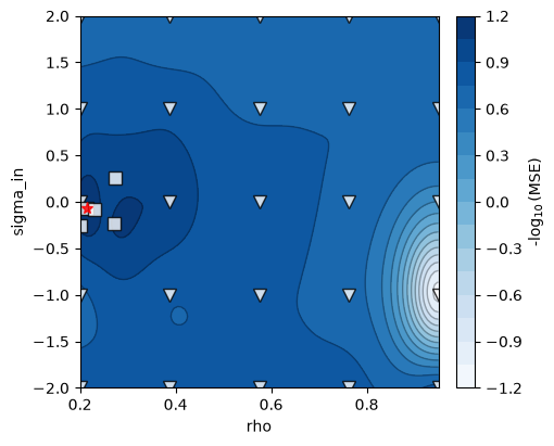
Validation-error landscape over
(rho, sigma_in)from tutorial 01: markers are the evaluated points (initial grid + gp-hedge acquisitions), the star the selected optimum.plot_training=Trueproduces this figure. 4. Solve the ridge regression for \(\mathbf{W}_\mathrm{out}\) on the full train + validation data with the selectedtikh.
training_summary() prints the realized split, folds, and selected
hyperparameters of the last call.
Seeded ensembles
The reservoir is a random draw, so train(n_seeds=m) trains m realizations
(seeds base, base+1, ...) in parallel processes, keeps the network with the
best validation score in place, and stores every score in seed_scores —
selection by validation score consistently lands in the ensemble's best half
on test error (see the
validation strategies page).
Forecasting
The ESN runs in two modes:
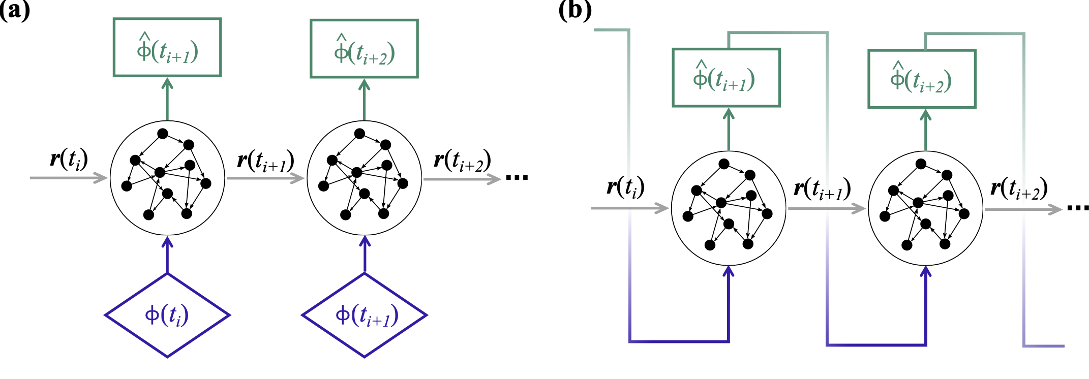
(a) open loop: the reservoir is driven by data \(\phi(t_i)\) and its readouts \(\hat{\phi}(t_{i+1})\) are one-step-ahead predictions; (b) closed loop: each prediction is fed back as the next input and the network runs autonomously.
- Open loop:
step()is fed observed data; used for training and for washout — driving the reservoir from \(\mathbf{r}_0 = \mathbf{0}\) through a short window of true history so it synchronizes with the physical state before a forecast. - Closed loop: each prediction is fed back as the next input
(
outputs_to_inputsselects the observed components and re-appends the parameter columns); the model runs autonomously.
r = np.zeros((esn.N_units, 1))
u = np.zeros((esn.N_dim, 1))
for u_in in wash:                      # open-loop washout on true history
    u, r = esn.step(u_in[:, None], r)

forecast = []
for _ in range(n_steps):               # closed-loop forecast
    u, r = esn.step(esn.outputs_to_inputs(u), r)
    forecast.append(u[:, 0])
Alignment: the washout's last output is the one-step-ahead prediction of the
frame after wash, so closed-loop prediction i corresponds to data row
len(wash) + 1 + i.
run_test() packages this — open-loop washout, closed-loop forecast, error
against truth — over the held-out test tail, with plots. For a fair error
metric across components use compute_nMAE(Y_true, Y_pred, norm=...), the
range-normalized mean absolute error used throughout training and validation.
See the EchoStateNetwork tutorial for the full workflow on Lorenz 63, and the API reference for every attribute and method.