Tutorial: validation strategies for chaotic time series
The ESN hyperparameters ($\rho$, $\sigma_\mathrm{in}$, the Tikhonov parameter $\lambda$) are selected by Bayesian optimization to minimize the closed-loop forecast error on validation data: the network is initialized open loop (washout on true data) and then run closed loop over a validation interval of $v$ steps,
$$ \epsilon(i) \;=\; \frac{1}{v} \sum_{n=i}^{i+v-1} \big\lVert \hat{\boldsymbol{y}}_n - \boldsymbol{y}_n \big\rVert^2 , $$
where $\hat{\boldsymbol{y}}_n$ is the prediction fed back as the next input and $\boldsymbol{y}_n$ the data. For a chaotic system this error is a fragile target: infinitesimally close trajectories separate as $\mathrm{e}^{\Lambda t}$, so $\epsilon(i)$ measured on a single interval behaves almost like a random draw — hyperparameters that happen to score well there need not generalize to the test data at all.
Racca & Magri (2021)
(arXiv:2103.03174) compare validation
strategies for ESNs on chaotic dynamics and show that the choice of strategy —
which data the hyperparameter search is allowed to see, and over how many
intervals the error is averaged — matters as much as the search itself. The
EchoStateNetwork class implements all four of their strategies:
| strategy | validation_strategy= |
$\boldsymbol{W}_\mathrm{out}$ during validation | validation intervals |
|---|---|---|---|
| single shot (SSV) | EchoStateNetwork._SSV |
trained once, on the data before the interval | 1 |
| walk forward (WFV) | EchoStateNetwork._WFV |
retrained per fold on a sliding window | $K$, tiling the end |
| K-fold (KFV) | EchoStateNetwork._KFV |
retrained per fold on all other data | $K$, tiling everything |
| recycle (RV) | default (_RVC_Noise) |
trained once on all the data — the same $\boldsymbol{W}_\mathrm{out}$ used at test time | $K$, inside the training data |
This tutorial reproduces the paper's partition schematic (their Figure 2), then
runs a live single-reservoir comparison of the four strategies on the Lorenz 63
system of the EchoStateNetwork class tutorial.
import matplotlib.pyplot as plt
import numpy as np
from scipy.integrate import solve_ivp

from echostatenetwork import EchoStateNetwork
How each strategy partitions the data
The schematic below -- redrawn after Figure 2 of Racca & Magri (2021), "Robust Optimization and Validation of Echo State Networks for learning chaotic dynamics", Neural Networks 142:252-268 (arXiv:2103.03174) -- shows how each strategy arranges unused, training and validation data along the time series. Each bar is one fold, i.e. one train/validate split contributing to the validation error the Bayesian search minimizes:
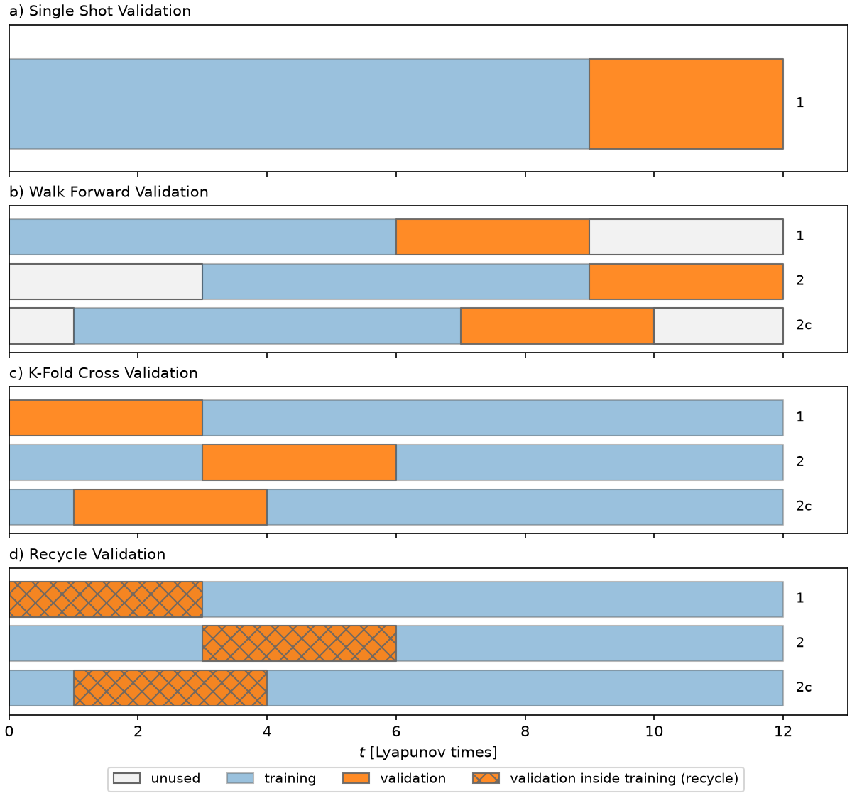
- bar 1 — the first fold;
- bar 2 — the second regular fold: the validation interval moves forward by its own length $v$;
- bar 2c — the second fold of the chaotic version: the validation interval moves forward by one Lyapunov time instead. Consecutive intervals overlap, but chaotic divergence ($\mathrm{e}^{\Lambda \cdot 1\,\mathrm{LT}} = \mathrm{e}$) decorrelates them enough to be informative — so many more validation intervals fit in the same data.
In every fold the reservoir is washed out open loop on the data immediately preceding the validation interval, then the closed-loop error is computed on the interval.
# Redrawn after Figure 2 of Racca & Magri (2021): v = 3 LT validation intervals
# on a 12 LT series; the 2c bars shift the second fold by 1 LT (chaotic version)
# instead of by v.
# STYLE = {
#     'unused': dict(facecolor='0.95', edgecolor='0.4'),
#     'train': dict(facecolor='tab:blue', alpha=0.45, edgecolor='0.4'),
#     'val': dict(facecolor='tab:orange', alpha=0.9, edgecolor='0.4'),
#     'val_in': dict(facecolor='tab:orange', alpha=0.9, edgecolor='0.4', hatch='xx'),
# }
# PANELS = {
#     'a) Single Shot Validation': [
#         [('train', 0, 9), ('val', 9, 12)]],
#     'b) Walk Forward Validation': [
#         [('train', 0, 6), ('val', 6, 9), ('unused', 9, 12)],
#         [('unused', 0, 3), ('train', 3, 9), ('val', 9, 12)],
#         [('unused', 0, 1), ('train', 1, 7), ('val', 7, 10), ('unused', 10, 12)]],
#     'c) K-Fold Cross Validation': [
#         [('val', 0, 3), ('train', 3, 12)],
#         [('train', 0, 3), ('val', 3, 6), ('train', 6, 12)],
#         [('train', 0, 1), ('val', 1, 4), ('train', 4, 12)]],
#     'd) Recycle Validation': [
#         [('train', 0, 12), ('val_in', 0, 3)],
#         [('train', 0, 12), ('val_in', 3, 6)],
#         [('train', 0, 12), ('val_in', 1, 4)]],
# }

# fig, axs = plt.subplots(4, 1, figsize=(8, 7.5), sharex=True, layout='constrained')
# for ax, (title, bars) in zip(axs, PANELS.items()):
#     for row, spans in enumerate(bars):
#         for kind, t0, t1 in spans:
#             ax.broken_barh([(t0, t1 - t0)], (-row - 0.4, 0.8), **STYLE[kind])
#         ax.text(12.2, -row, '1' if row == 0 else ('2' if row == 1 else '2c'),
#                 va='center', fontsize=9)
#     ax.set_title(title, loc='left', fontsize=10)
#     ax.set(yticks=[], ylim=(-len(bars) + 0.4, 0.7), xlim=(0, 13))
# axs[-1].set_xlabel('$t$ [Lyapunov times]')
# handles = [plt.Rectangle((0, 0), 1, 1, **STYLE[k]) for k in STYLE]
# fig.legend(handles, ['unused', 'training', 'validation',
#                      'validation inside training (recycle)'],
#            loc='outside lower center', ncols=4, fontsize=9)
# plt.show()

What the figure conveys, strategy by strategy:
- SSV tunes the hyperparameters on one small interval at the end of the data. For a chaotic signal that single number is a poor proxy for test performance — this is the strategy the paper warns against.
- WFV distributes the validation over several intervals that tile the end of the data, sliding a fixed-length training window forward by $v$ per fold and retraining $\boldsymbol{W}_\mathrm{out}$ on each window. Only causal (past $\to$ future) splits are used.
- KFV goes further: the intervals tile all the data, and each fold trains on everything outside its own interval — more data per fold than WFV, but still one retraining per fold, and the early folds validate on data that precedes most of their training set.
- RV (recycle) trains $\boldsymbol{W}_\mathrm{out}$ once, on all $n$ points — exactly the $\boldsymbol{W}_\mathrm{out}$ that will be used at test time — and re-uses ("recycles") intervals inside the training data for closed-loop validation. The validation data is not held out, yet the paper shows RV selects hyperparameters as well as KFV at a fraction of the cost: no per-fold retraining, and no data sacrificed — the advantage grows on small datasets.
- The 2c bars are the chaotic versions ($\mathrm{SSV}$ has none — it has
a single interval by definition): shifting the folds by 1 LT instead of $v$
multiplies the number of validation intervals the error is averaged over.
In this package the fold shift is the
val_fold_stepattribute (in ESN steps; the defaultNonekeeps the regular non-overlapping folds), e.g.EchoStateNetwork(..., val_fold_step=N_LYAP)turns_WFV/_KFVinto their chaotic versions. The package default,_RVC_Noise, is exactly this chaotic recycle validation (with noise regularization of the training inputs).
Live comparison on the Lorenz 63 system
One reservoir, four hyperparameter searches. We deliberately mirror the paper's small-data setup (their Sec. 4): about 12 Lyapunov times of washout+train+validation data, $N_\mathrm{units} = 100$, and a small Bayesian search (15 evaluations) over $\rho \in [0.1, 1]$ and $\sigma_\mathrm{in} \in [0.5, 5]$, with the Tikhonov parameter selected per fold from $\{10^{-9}, 10^{-11}\}$. The reservoir ($\boldsymbol{W}$, $\boldsymbol{W}_\mathrm{in}$, i.e. the seed) is identical in the four trainings — only the validation strategy seen by the search differs. With so little data the choice has to matter.
T_LYAP = 1 / 0.906                    # Lyapunov time of the Lorenz 63 system
DT = 0.02
N_LYAP = int(T_LYAP / DT)             # ESN steps per Lyapunov time


def lorenz63(dt, n_lyap_times, noise_level=0.005, seed=0):
    """Noisy and clean Lorenz 63 trajectories on the attractor."""
    def rhs(t, u):
        return [10 * (u[1] - u[0]), u[0] * (28 - u[2]) - u[1],
                u[0] * u[1] - 8 / 3 * u[2]]
    t_end = (n_lyap_times + 10) * T_LYAP
    sol = solve_ivp(rhs, [0, t_end], [1., 1., 1.], t_eval=np.arange(0, t_end, dt),
                    method='RK45', rtol=1e-9)
    clean = sol.y.T[int(10 * T_LYAP / dt):]          # discard the transient
    rng = np.random.default_rng(seed)
    return clean + noise_level * clean.std(axis=0) * rng.standard_normal(clean.shape), clean


noisy, clean = lorenz63(DT, 22)
N_train, N_val = 9 * N_LYAP, 3 * N_LYAP
train_val_data = noisy[:N_train + N_val]   # 12 LT: washout + training + validation
test_clean = clean[N_train + N_val:]       # 10 LT held out for closed-loop testing
print(f'train+val: {train_val_data.shape[0]} steps, test: {test_clean.shape[0]} steps')
train+val: 660 steps, test: 556 steps
ESN_PARAMS = dict(N_wash=N_LYAP,           # 1 LT open-loop washout
                  N_units=100, upsample=1, seed=0,
                  t_train=N_train * DT, t_val=N_val * DT, t_test=0.,
                  N_func_evals=15, N_grid=3, noise=1e-2,
                  N_folds=3,
                  rho_range=(.1, 1.),                              # paper Sec. 4
                  sigma_in_range=(np.log10(0.5), np.log10(5.)),    # log10 axis
                  tikh_range=[1e-9, 1e-11])

ESN_init = EchoStateNetwork(train_val_data.T, dt=DT, **ESN_PARAMS)

STRATEGIES = {'SSV (single shot)': EchoStateNetwork._SSV,
              'WFV (walk forward)': EchoStateNetwork._WFV,
              'KFV (K-fold)': EchoStateNetwork._KFV,
              'RV (recycle, default)': None}   # None -> the default _RVC_Noise
N_folds=3 gives WFV and KFV the three non-overlapping intervals of length
t_val that fit in the data. The recycle strategy validates inside the
training data with chaotic (overlapping) fold placement, so it can afford more
intervals from the same series — we give it N_folds=6 at its train call.
Each training prints its training_summary().
esns = {}
for name, strategy in STRATEGIES.items():
    print(f'{"-" * 21} {name} {"-" * (36 - len(name))}')
    esn = ESN_init.copy()      # identical reservoir: only the validation strategy differs
    esn.train(train_val_data, plot_training=False, validation_strategy=strategy,
              **(dict(N_folds=6) if name.startswith('RV') else {}))
    esns[name] = esn
--------------------- SSV (single shot) -------------------
seed 0 	 Optimal hyperparameters: [1.0, 0.6946342849299372], 1e-11, val score: -1.6867075379319256
trained: 495+165 train+val steps, 0 test | t_train=9.9, t_val=3.3 | rho=1, sigma_in=4.95, tikh=1e-11 | 1 validation fold | BHO: 15 evals over ['rho', 'sigma_in']
--------------------- WFV (walk forward) ------------------
seed 0 	 Optimal hyperparameters: [0.10545001852059734, 0.21645251275603233], 1e-09, val score: -0.5670303604728543
trained: 495+165 train+val steps, 0 test | t_train=9.9, t_val=3.3 | rho=0.105, sigma_in=1.65, tikh=1e-09 | 3 validation folds | BHO: 15 evals over ['rho', 'sigma_in']
--------------------- KFV (K-fold) ------------------------
seed 0 	 Optimal hyperparameters: [0.1142787674360431, 0.18575187053654935], 1e-11, val score: -1.6515583662783488
trained: 495+165 train+val steps, 0 test | t_train=9.9, t_val=3.3 | rho=0.114, sigma_in=1.53, tikh=1e-11 | 3 validation folds | BHO: 15 evals over ['rho', 'sigma_in']
--------------------- RV (recycle, default) ---------------
Modifying N_folds = 3 -> 6 at training.
seed 0 	 Optimal hyperparameters: [0.5547002809121359, 0.017174507131998362], 1e-11, val score: -1.9644468586440285
trained: 495+165 train+val steps, 0 test | t_train=9.9, t_val=3.3 | rho=0.555, sigma_in=1.04, tikh=1e-11 | 6 validation folds | BHO: 15 evals over ['rho', 'sigma_in']
Closed-loop forecasts on unseen data
Each trained ESN is initialized open loop on the same 1-Lyapunov-time washout of (clean) test data, then run closed loop from the same test start. The predictability horizon in each panel title is the time until the normalized error first exceeds 0.2 (the paper's threshold), in Lyapunov times.
def closed_loop(esn, wash, n_steps):
    """Open-loop washout on true history, then an n_steps closed-loop forecast.

    The washout drives the reservoir open loop through `wash`; its last output
    (the one-step-ahead prediction of the frame after `wash`) is the first
    closed-loop input, so prediction i corresponds to the data row
    len(wash) + 1 + i — as in scripts/compare_validation_strategies.py."""
    r = np.zeros((esn.N_units, 1))
    u = np.zeros((esn.N_dim, 1))
    for u_in in wash:
        u, r = esn.step(u_in[:, None], r)
    U = []
    for _ in range(n_steps):
        u, r = esn.step(esn.outputs_to_inputs(u), r)
        U.append(u[:, 0])
    return np.array(U)


def forecast_and_horizon(esn, i0, n_fc, threshold=0.2):
    """Forecast n_fc steps from test start i0; horizon in Lyapunov times."""
    truth = test_clean[i0 + N_LYAP + 1:i0 + N_LYAP + 1 + n_fc]
    U = closed_loop(esn, test_clean[i0:i0 + N_LYAP], len(truth))
    err = np.linalg.norm((U - truth) / test_clean.std(axis=0), axis=1) / np.sqrt(3)
    above = np.flatnonzero(err > threshold)
    return U, truth, (above[0] if above.size else len(truth)) * DT / T_LYAP


n_fc = 6 * N_LYAP
t_fc = np.arange(n_fc) * DT / T_LYAP

fig, axs = plt.subplots(4, 1, sharex=True, sharey=True, figsize=(8, 7.5),
                        layout='tight')
for ax, (name, esn) in zip(axs, esns.items()):
    U, truth, h = forecast_and_horizon(esn, i0=0, n_fc=n_fc)
    ax.plot(t_fc, truth[:, 0], 'k', lw=1.4, label='truth')
    ax.plot(t_fc, U[:, 0], 'C3', lw=1.1, label='closed-loop forecast')
    ax.axvline(h, color='0.4', dashes=[4, 2], lw=1)
    ax.set(ylabel='$x$', title=f'{name}: predictability horizon {h:.2f} Lyapunov times')
    ax.grid(alpha=0.3)
axs[0].legend(ncols=2, fontsize=9, loc='upper right')
axs[-1].set(xlabel='$t$ [Lyapunov times]')
plt.show()

A single forecast is itself a single draw from the chaotic system — the honest comparison averages the horizon over several test starts:
for name, esn in esns.items():
    hs = [forecast_and_horizon(esn, i0=s * 80, n_fc=n_fc)[2] for s in range(5)]
    print(f'{name:24s} mean horizon over 5 test starts: {np.mean(hs):.2f} LT  '
          + str([f'{h:.1f}' for h in hs]))
SSV (single shot)        mean horizon over 5 test starts: 0.63 LT  ['1.0', '0.5', '0.5', '0.4', '0.8']
WFV (walk forward)       mean horizon over 5 test starts: 1.80 LT  ['1.1', '3.3', '1.7', '0.5', '2.4']
KFV (K-fold)             mean horizon over 5 test starts: 1.76 LT  ['1.1', '3.2', '1.7', '0.5', '2.3']
RV (recycle, default)    mean horizon over 5 test starts: 1.80 LT  ['1.2', '3.2', '1.8', '0.5', '2.3']
The paper's headline number: validation–test correlation
A validation strategy is only as good as the agreement between the error it reports and the error at test time. Table 1 of Racca & Magri (2021) quantifies this as the Spearman correlation between validation MSE and test MSE over an ensemble of $50$ reservoir realizations (each with its own optimal hyperparameters), for a short ($12$ LT) and a long ($24$ LT) dataset (subscript $c$ = chaotic version):
| strategy | short (12 LT) | long (24 LT) |
|---|---|---|
| SSV | 0.31 | 0.49 |
| WFV | 0.31 | 0.51 |
| WFV$_c$ | 0.50 | 0.61 |
| KFV | 0.60 | 0.70 |
| KFV$_c$ | 0.65 | 0.85 |
| RV | 0.59 | 0.67 |
| RV$_c$ | 0.62 | 0.81 |
Three consistent messages: SSV correlates worst with the test error; every chaotic version beats its regular counterpart (more validation intervals from the same data); and KFV$_c$ is best, with RV$_c$ close behind at recycle cost — a single training, no per-fold retraining, no held-out data.
scripts/compare_validation_strategies.py
is the runnable ensemble version of this comparison: for an ensemble of
reservoir seeds it records each member's best validation error alongside its
test MSE — the (validation, test) pairs behind this same table and the
paper's Fig. 8 validation-vs-test scatter.
Seeded ensembles: train(n_seeds=...)
Everything above used one reservoir realization per strategy (seed=0), but
W and W_in are random draws -- Racca & Magri's tables are ensemble
statements precisely because a single draw can be lucky or unlucky.
train(n_seeds=m) trains m realizations of the same ESN (seeds
base, base+1, ...) on the same data and settings, one process each, scores
every one with the validation strategy (the BHO minimum), keeps the best
network in place, and stores all the scores in seed_scores for the
statistical comparison.
Selecting by validation score works: in the ensemble run of
scripts/compare_validation_strategies.py
the kept member always lands in the ensemble's best half on test error,
usually the best quarter -- and recycle validation on the short dataset picked
the true best of 96 seeds.
esn_ens = ESN_init.copy()
esn_ens.train(train_val_data, plot_training=False, n_seeds=4, N_folds=6)  # default RV_c

print('log10 validation score per seed:',
      ', '.join(f'{s}: {v:.3f}' for s, v in esn_ens.seed_scores.items()))
hs = [forecast_and_horizon(esn_ens, i0=s * 80, n_fc=n_fc)[2] for s in range(5)]
print(f'kept network (seed {esn_ens.seed}): '
      f'mean horizon over 5 test starts {np.mean(hs):.2f} LT')
Modifying N_folds = 3 -> 6 at training.
seed 0 	 Optimal hyperparameters: [0.48774092508204236, 0.26124391817825504], 1e-09, val score: -1.9179080712341385
trained: 495+165 train+val steps, 0 test | t_train=9.9, t_val=3.3 | rho=0.488, sigma_in=1.82, tikh=1e-09 | 6 validation folds | BHO: 15 evals over ['rho', 'sigma_in']
Modifying N_folds = 3 -> 6 at training.
seed 1 	 Optimal hyperparameters: [0.5968594368114074, 0.04777031226446771], 1e-09, val score: -1.6186088863032069
trained: 495+165 train+val steps, 0 test | t_train=9.9, t_val=3.3 | rho=0.597, sigma_in=1.12, tikh=1e-09 | 6 validation folds | BHO: 15 evals over ['rho', 'sigma_in']
Modifying N_folds = 3 -> 6 at training.
seed 2 	 Optimal hyperparameters: [0.49058376540430426, -0.012128485141530199], 1e-11, val score: -1.6481693856381143
trained: 495+165 train+val steps, 0 test | t_train=9.9, t_val=3.3 | rho=0.491, sigma_in=0.972, tikh=1e-11 | 6 validation folds | BHO: 15 evals over ['rho', 'sigma_in']
Modifying N_folds = 3 -> 6 at training.
seed 3 	 Optimal hyperparameters: [0.3900357616047393, -0.02289948163074268], 1e-11, val score: -1.534807178399891
trained: 495+165 train+val steps, 0 test | t_train=9.9, t_val=3.3 | rho=0.39, sigma_in=0.949, tikh=1e-11 | 6 validation folds | BHO: 15 evals over ['rho', 'sigma_in']
n_seeds=4: validation score -1.6799 +/- 0.1436 (best -1.9179 @ seed 0, worst -1.5348) -> kept seed 0
log10 validation score per seed: 0: -1.918, 1: -1.619, 2: -1.648, 3: -1.535
kept network (seed 0): mean horizon over 5 test starts 1.50 LT