Skip to content

Annular combustor

The annular combustor model extends the single-mode picture of the Van der Pol and Rijke models to the first azimuthal mode pair of an annular geometry, such as a gas-turbine combustion chamber. Decomposing the acoustic pressure as \(p(\theta,t) = \eta_a(t)\cos(\theta) + \eta_b(t)\sin(\theta)\) gives four coupled first-order ODEs for \((\eta_a, \dot{\eta}_a, \eta_b, \dot{\eta}_b)\), with a growth rate \(\nu\), a resistive asymmetry \(c_2\beta\), a saturation \(\kappa\), and a reactive asymmetry \((\epsilon, \Theta_\epsilon)\) that breaks the rotational symmetry of an idealized annulus. The full equations are in the API reference below.

The balance between \(\nu\) and \(c_2\beta\) sets the qualitative regime. Three named cases are pre-tabulated in CASES and selected with case='...' (explicit keyword arguments override a case's values); the class defaults (ER=0.5) give \(\nu<0\), a linearly stable mode that decays to the origin rather than self-oscillating, so pick a case (or set nu/c2beta explicitly) for a self-sustained oscillation.

Quickstart

from dynamodels.physical import Annular

model = Annular(case='mixed', dt=1./51200)
psi, t = model.time_integrate(Nt=30000)
model.update_history(psi, t)
model.visualize_observable_hist()
model.close()

Annular.nu_from_ER(ER) and Annular.c2beta_from_ER(ER) map an equivalence ratio to \((\nu, c_2\beta)\) along the calibrated experimental trend, in case neither a case nor explicit values fit.

Regimes
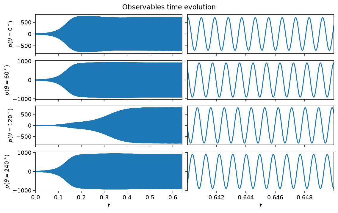
Annular combustor, spinning mode

case='spinning', \((\nu, c_2\beta) = (30, 5)\): growing onto a self-sustained oscillation. With \(c_2\beta\) small relative to \(\nu\), the pattern rotates around the annulus rather than sitting still, so the four microphones' final amplitudes are closer to each other than in the standing case below (the small residual spread comes from the model's built-in reactive asymmetry, \(\epsilon\)).
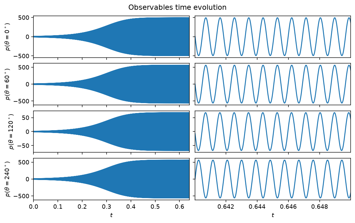
Annular combustor, standing mode

case='standing', \((\nu, c_2\beta) = (0, 50)\): a fixed node-antinode pattern rather than a rotating one. The \(\theta=120^\circ\) microphone sits almost exactly on a node, with roughly an order of magnitude smaller amplitude than the other three.
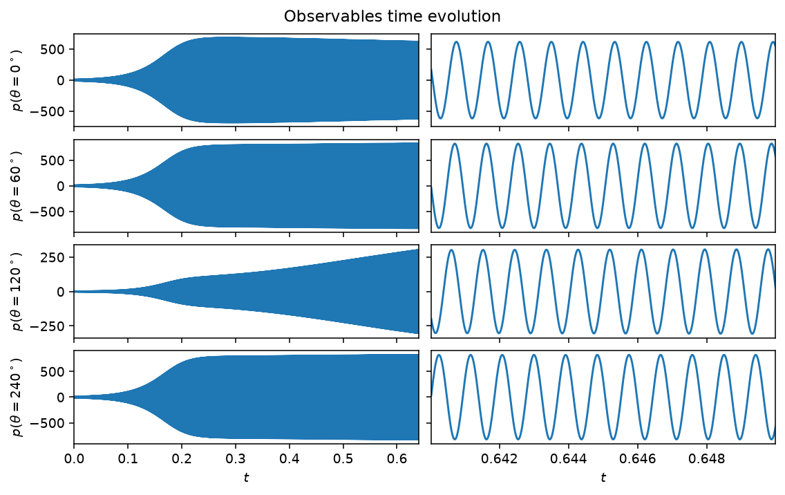
Annular combustor, mixed mode

case='mixed', \((\nu, c_2\beta) = (20, 18)\), past the transient. Left: the full run. Right: a few periods of the established oscillation. The \(\theta=120^\circ\) microphone sits closer to a pressure node of this mode and saturates more slowly.

A microphone trace alone does not show where the pressure pattern sits around the annulus, nor whether it rotates. An animation does:
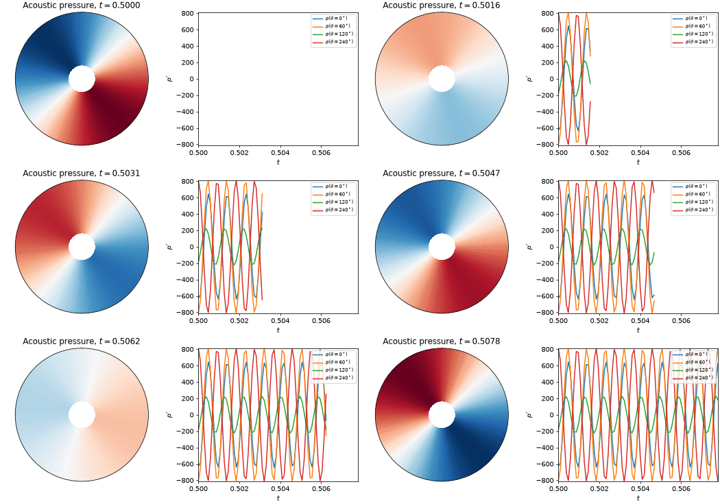
Annular combustor, mixed mode, animated

case='mixed', past the transient. Left: the acoustic pressure \(p(\theta,t) = \eta_a\cos\theta + \eta_b\sin\theta\) around the annulus, with \(\theta=0^\circ\) at the top. Right: the same field sampled at the four microphones. The pattern neither stands still nor rotates steadily: it is the mixed state between the two limits above. The annular combustor tutorial builds this figure step by step.

Nonlinear diagnostics

ntsa characterization of Annular

Diagnostics from ntsa.characterize on the mixed mode, left to right: the observable time series with a zoomed inset; power spectral density; the 3-D delay-embedded portrait; the first-return map of the maxima; a plane-crossing Poincare section; a recurrence plot; a 3-D classical-MDS embedding of the full state; and the leading Lyapunov exponent.

Reference

Novoa, A., Noiray, N., Dawson, J. R., & Magri, L. (2024). A real-time digital twin of azimuthal thermoacoustic instabilities. Journal of Fluid Mechanics, 1001, A49. doi:10.1017/jfm.2024.1052

API

dynamodels.physical.annular.Annular

Bases: Model

Annular combustor — two coupled oscillators for the first azimuthal modes.

The acoustic pressure in the annulus obeys the wave equation with heat-release source and resistive/reactive asymmetries,

\[ \frac{\partial^2 p}{\partial t^2} + \zeta \frac{\partial p}{\partial t} - \left[ 1 + \epsilon \cos\!\big(2(\theta - \Theta_\epsilon)\big) \right] \frac{c^2}{r^2} \frac{\partial^2 p}{\partial \theta^2} = (\gamma - 1)\, \frac{\partial \dot{q}}{\partial t}, \qquad (\gamma - 1)\, \dot{q} = \beta \left[ 1 + c_2 \cos\!\big(2(\theta - \Theta_\beta)\big) \right] p - \kappa p^3 . \]

Decomposing the pressure field onto the first azimuthal mode pair (\(n = 1\)),

\[ p(\theta, t) = \eta_a(t) \cos(n\theta) + \eta_b(t) \sin(n\theta), \]

yields four coupled first-order ODEs for \((\eta_a, \dot{\eta}_a, \eta_b, \dot{\eta}_b)\):

\[ \ddot{\eta}_a = -\omega^2 \left[ \eta_a \big(1 + \tfrac{\epsilon}{2} \cos 2\Theta_\epsilon\big) + \eta_b \tfrac{\epsilon}{2} \sin 2\Theta_\epsilon \right] + \dot{\eta}_a \left[ 2\nu + \tfrac{c_2\beta}{2} \cos 2\Theta_\beta - \tfrac{3\kappa}{4} (3\eta_a^2 + \eta_b^2) \right] + \dot{\eta}_b \left[ \tfrac{c_2\beta}{2} \sin 2\Theta_\beta - \tfrac{3\kappa}{2} \eta_a \eta_b \right], \]
\[ \ddot{\eta}_b = -\omega^2 \left[ \eta_b \big(1 - \tfrac{\epsilon}{2} \cos 2\Theta_\epsilon\big) + \eta_a \tfrac{\epsilon}{2} \sin 2\Theta_\epsilon \right] + \dot{\eta}_b \left[ 2\nu - \tfrac{c_2\beta}{2} \cos 2\Theta_\beta - \tfrac{3\kappa}{4} (3\eta_b^2 + \eta_a^2) \right] + \dot{\eta}_a \left[ \tfrac{c_2\beta}{2} \sin 2\Theta_\beta - \tfrac{3\kappa}{2} \eta_a \eta_b \right]. \]

The estimable parameters are the growth rate \(\nu\), the resistive-asymmetry intensity \(c_2\beta\), the saturation \(\kappa\), the reactive-asymmetry amplitude \(\epsilon\) and phase \(\Theta_\epsilon\), the frequency \(\omega\) and the direction of maximum r.m.s. pressure \(\Theta_\beta\).

Three named regimes are pre-tabulated in CASES and selected with case='...' (explicit keyword arguments override a case's values):

  • 'spinning': purely spinning mode, \((\nu, c_2\beta) = (30, 5)\);
  • 'standing': purely standing mode, \((\nu, c_2\beta) = (0, 50)\);
  • 'mixed': mixed mode, \((\nu, c_2\beta) = (20, 18)\).

The class defaults (ER=0.5) give \(\nu<0\), a linearly stable mode that decays to the origin rather than self-oscillating; use a case or set nu/c2beta explicitly for a self-sustained oscillation.

References

Nóvoa, Noiray, Dawson & Magri (2024). A real-time digital twin of azimuthal thermoacoustic instabilities. J. Fluid Mech., 1001, A49. DOI: 10.1017/jfm.2024.1052.

Source code in dynamodels/physical/annular.py
 17
 18
 19
 20
 21
 22
 23
 24
 25
 26
 27
 28
 29
 30
 31
 32
 33
 34
 35
 36
 37
 38
 39
 40
 41
 42
 43
 44
 45
 46
 47
 48
 49
 50
 51
 52
 53
 54
 55
 56
 57
 58
 59
 60
 61
 62
 63
 64
 65
 66
 67
 68
 69
 70
 71
 72
 73
 74
 75
 76
 77
 78
 79
 80
 81
 82
 83
 84
 85
 86
 87
 88
 89
 90
 91
 92
 93
 94
 95
 96
 97
 98
 99
100
101
102
103
104
105
106
107
108
109
110
111
112
113
114
115
116
117
118
119
120
121
122
123
124
125
126
127
128
129
130
131
132
133
134
135
136
137
138
139
140
141
142
143
144
145
146
147
148
149
150
151
152
153
154
155
156
157
158
159
160
161
162
163
164
165
166
167
168
169
170
171
172
173
174
175
176
177
178
179
180
181
182
183
184
185
186
187
188
189
190
191
192
193
194
195
196
197
198
199
200
201
202
203
class Annular(Model):
    r"""Annular combustor — two coupled oscillators for the first azimuthal modes.

    The acoustic pressure in the annulus obeys the wave equation with heat-release
    source and resistive/reactive asymmetries,

    $$
    \frac{\partial^2 p}{\partial t^2} + \zeta \frac{\partial p}{\partial t}
    - \left[ 1 + \epsilon \cos\!\big(2(\theta - \Theta_\epsilon)\big) \right]
    \frac{c^2}{r^2} \frac{\partial^2 p}{\partial \theta^2}
    = (\gamma - 1)\, \frac{\partial \dot{q}}{\partial t},
    \qquad
    (\gamma - 1)\, \dot{q} = \beta \left[ 1 + c_2
    \cos\!\big(2(\theta - \Theta_\beta)\big) \right] p - \kappa p^3 .
    $$

    Decomposing the pressure field onto the first azimuthal mode pair
    ($n = 1$),

    $$
    p(\theta, t) = \eta_a(t) \cos(n\theta) + \eta_b(t) \sin(n\theta),
    $$

    yields four coupled first-order ODEs for
    $(\eta_a, \dot{\eta}_a, \eta_b, \dot{\eta}_b)$:

    $$
    \ddot{\eta}_a = -\omega^2 \left[ \eta_a \big(1 + \tfrac{\epsilon}{2}
    \cos 2\Theta_\epsilon\big) + \eta_b \tfrac{\epsilon}{2} \sin 2\Theta_\epsilon \right]
    + \dot{\eta}_a \left[ 2\nu + \tfrac{c_2\beta}{2} \cos 2\Theta_\beta
    - \tfrac{3\kappa}{4} (3\eta_a^2 + \eta_b^2) \right]
    + \dot{\eta}_b \left[ \tfrac{c_2\beta}{2} \sin 2\Theta_\beta
    - \tfrac{3\kappa}{2} \eta_a \eta_b \right],
    $$

    $$
    \ddot{\eta}_b = -\omega^2 \left[ \eta_b \big(1 - \tfrac{\epsilon}{2}
    \cos 2\Theta_\epsilon\big) + \eta_a \tfrac{\epsilon}{2} \sin 2\Theta_\epsilon \right]
    + \dot{\eta}_b \left[ 2\nu - \tfrac{c_2\beta}{2} \cos 2\Theta_\beta
    - \tfrac{3\kappa}{4} (3\eta_b^2 + \eta_a^2) \right]
    + \dot{\eta}_a \left[ \tfrac{c_2\beta}{2} \sin 2\Theta_\beta
    - \tfrac{3\kappa}{2} \eta_a \eta_b \right].
    $$

    The estimable parameters are the growth rate $\nu$, the resistive-asymmetry
    intensity $c_2\beta$, the saturation $\kappa$, the reactive-asymmetry amplitude
    $\epsilon$ and phase $\Theta_\epsilon$, the frequency $\omega$ and the
    direction of maximum r.m.s. pressure $\Theta_\beta$.

    Three named regimes are pre-tabulated in `CASES` and selected with
    ``case='...'`` (explicit keyword arguments override a case's values):

    - ``'spinning'``: purely spinning mode, $(\nu, c_2\beta) = (30, 5)$;
    - ``'standing'``: purely standing mode, $(\nu, c_2\beta) = (0, 50)$;
    - ``'mixed'``: mixed mode, $(\nu, c_2\beta) = (20, 18)$.

    The class defaults (`ER=0.5`) give $\nu<0$, a linearly stable mode that
    decays to the origin rather than self-oscillating; use a `case` or set
    `nu`/`c2beta` explicitly for a self-sustained oscillation.

    References
    ----------
    Nóvoa, Noiray, Dawson & Magri (2024). A real-time digital twin of azimuthal
    thermoacoustic instabilities. *J. Fluid Mech.*, 1001, A49.
    [DOI: 10.1017/jfm.2024.1052](https://doi.org/10.1017/jfm.2024.1052).
    """

    t_transient = 0.5
    t_CR = 0.01

    ER = 0.5
    nu_1, nu_2 = 633.77, -331.39
    c2b_1, c2b_2 = 258.3, -108.27  # values in Matlab codes

    Nq = 4
    theta_mic = np.radians([0, 60, 120, 240])


    theta_b = 0.63
    theta_e = 0.66
    omega = 1090 * 2 * np.pi
    epsilon = 2.3E-3

    nu = nu_1 * ER + nu_2
    c2beta = c2b_1 * ER + c2b_2
    kappa = 1.2E-4
    params = ['omega', 'nu', 'c2beta', 'kappa', 'epsilon', 'theta_b', 'theta_e']

    # __________________________ Init method ___________________________ #
    def __init__(self, **model_dict):

        case = model_dict.pop('case', None)
        if case is not None:
            if case not in CASES:
                raise ValueError(f"Unknown case '{case}'. Must be one of {list(CASES)}.")
            for key, val in CASES[case].items():
                model_dict.setdefault(key, val)  # explicit kwargs win over the case

        dt = model_dict.pop('dt', 1. / 51200)
        psi0 = model_dict.pop('psi0', None)
        if psi0 is None:
            C0, X0, th0, ph0 = 10, 0, 0.63, 0  # %initial values
            # Conversion of the initial conditions from the quaternion formalism to the AB formalism
            Ai = C0 * np.sqrt(np.cos(th0) ** 2 * np.cos(X0) ** 2 + np.sin(th0) ** 2 * np.sin(X0) ** 2)
            Bi = C0 * np.sqrt(np.sin(th0) ** 2 * np.cos(X0) ** 2 + np.cos(th0) ** 2 * np.sin(X0) ** 2)
            phai = ph0 + np.arctan2(np.sin(th0) * np.sin(X0), np.cos(th0) * np.cos(X0))
            phbi = ph0 - np.arctan2(np.cos(th0) * np.sin(X0), np.sin(th0) * np.cos(X0))

            # %initial conditions for the fast oscillator equations
            psi0 = [Ai * np.cos(phai),
                    -self.omega * Ai * np.sin(phai),
                    Bi * np.cos(phbi),
                    -self.omega * Bi * np.sin(phbi)]

            psi0 = np.array(psi0)  # initialise \eta_a, \dot{\eta_a}, \eta_b, \dot{\eta_b}

        super().__init__(psi0=psi0, dt=dt, integrator_class=IVPIntegrator, **model_dict)

        self.alpha_labels = dict(omega='$\\omega$', nu='$\\nu$', c2beta='$c_2\\beta $', kappa='$\\kappa$',
                                 epsilon='$\\epsilon$', theta_b='$\\Theta_\\beta$', theta_e='$\\Theta_\\epsilon$')

        self.alpha_lims =  dict(omega=(1000 * 2 * np.pi, 1300 * 2 * np.pi),
                                nu=(-60., 100.), c2beta=(0., 100.),
                                theta_b=(0, 2 * np.pi), theta_e=(0, 2 * np.pi))

    # _______________  Specific properties and methods ________________ #
    @property
    def obs_labels(self, loc=None, measure_modes=False):
        if measure_modes:
            return ["$\\eta_1$", '$\\eta_2$']
        else:
            if loc is None:
                loc = self.theta_mic
            return [f"$p(\\theta={int(np.round(np.degrees(th)))}^\\circ)$" for th in np.array(loc)]
    @property
    def state_labels(self):
        return  ['$\\eta_{a}$', '$\\dot{\\eta}_{a}$', '$\\eta_{b}$', '$\\dot{\\eta}_{b}$']


    @staticmethod
    def nu_from_ER(ER):
        return Annular.nu_1 * ER + Annular.nu_2

    @staticmethod
    def c2beta_from_ER(ER):
        return Annular.c2b_1 * ER + Annular.c2b_2

    def get_observables(self, Nt=1, loc=None, measure_modes=False, **kwargs):
        """
        pressure measurements at theta = [0º, 60º, 120º, 240º]
        """
        if loc is None:
            loc = self.theta_mic

        if measure_modes:
            return self.hist[-Nt:, [0, 2], :]
        else:
            eta1, eta2 = self.hist[-Nt:, 0, :], self.hist[-Nt:, 2, :]
            if max(loc) > 2 * np.pi:
                raise ValueError('Theta must be in radians')

            p_mics = np.array([eta1 * np.cos(th) + eta2 * np.sin(th) for th in np.array(loc)])
            p_mics = p_mics.transpose(1, 0, 2)
            if Nt == 1:
                return p_mics.squeeze(axis=0)
            else:
                return p_mics

    @staticmethod
    def time_derivative(t, psi, nu, kappa, c2beta, theta_b, omega, epsilon, theta_e):
        """Time derivative of the two coupled azimuthal oscillators (see class docstring)."""
        y_a, z_a, y_b, z_b = psi[:4]  # y = η, and z = dη/dt

        def k1(y1, y2, sign):
            return (2 * nu - 3. / 4 * kappa * (3 * y1 ** 2 + y2 ** 2) +
                    sign * c2beta / 2. * np.cos(2. * theta_b))

        k2 = c2beta / 2. * np.sin(2. * theta_b) - 3. / 2 * kappa * y_a * y_b

        def k3(y1, y2, sign):
            return omega ** 2 * (y1 * (1 + sign * epsilon / 2. * np.cos(2. * theta_e)) +
                                 y2 * epsilon / 2. * np.sin(2. * theta_e))

        dz_a = z_a * k1(y_a, y_b, sign=1) + z_b * k2 - k3(y_a, y_b, sign=1)
        dz_b = z_b * k1(y_b, y_a, sign=-1) + z_a * k2 - k3(y_b, y_a, sign=-1)

        return (z_a, dz_a, z_b, dz_b) + (0,) * (len(psi) - 4)

get_observables(Nt=1, loc=None, measure_modes=False, **kwargs)

pressure measurements at theta = [0º, 60º, 120º, 240º]

Source code in dynamodels/physical/annular.py
164
165
166
167
168
169
170
171
172
173
174
175
176
177
178
179
180
181
182
183
def get_observables(self, Nt=1, loc=None, measure_modes=False, **kwargs):
    """
    pressure measurements at theta = [0º, 60º, 120º, 240º]
    """
    if loc is None:
        loc = self.theta_mic

    if measure_modes:
        return self.hist[-Nt:, [0, 2], :]
    else:
        eta1, eta2 = self.hist[-Nt:, 0, :], self.hist[-Nt:, 2, :]
        if max(loc) > 2 * np.pi:
            raise ValueError('Theta must be in radians')

        p_mics = np.array([eta1 * np.cos(th) + eta2 * np.sin(th) for th in np.array(loc)])
        p_mics = p_mics.transpose(1, 0, 2)
        if Nt == 1:
            return p_mics.squeeze(axis=0)
        else:
            return p_mics

time_derivative(t, psi, nu, kappa, c2beta, theta_b, omega, epsilon, theta_e) staticmethod

Time derivative of the two coupled azimuthal oscillators (see class docstring).

Source code in dynamodels/physical/annular.py
185
186
187
188
189
190
191
192
193
194
195
196
197
198
199
200
201
202
203
@staticmethod
def time_derivative(t, psi, nu, kappa, c2beta, theta_b, omega, epsilon, theta_e):
    """Time derivative of the two coupled azimuthal oscillators (see class docstring)."""
    y_a, z_a, y_b, z_b = psi[:4]  # y = η, and z = dη/dt

    def k1(y1, y2, sign):
        return (2 * nu - 3. / 4 * kappa * (3 * y1 ** 2 + y2 ** 2) +
                sign * c2beta / 2. * np.cos(2. * theta_b))

    k2 = c2beta / 2. * np.sin(2. * theta_b) - 3. / 2 * kappa * y_a * y_b

    def k3(y1, y2, sign):
        return omega ** 2 * (y1 * (1 + sign * epsilon / 2. * np.cos(2. * theta_e)) +
                             y2 * epsilon / 2. * np.sin(2. * theta_e))

    dz_a = z_a * k1(y_a, y_b, sign=1) + z_b * k2 - k3(y_a, y_b, sign=1)
    dz_b = z_b * k1(y_b, y_a, sign=-1) + z_a * k2 - k3(y_b, y_a, sign=-1)

    return (z_a, dz_a, z_b, dz_b) + (0,) * (len(psi) - 4)