Lorenz63

The Lorenz (1963) system is the standard low-order benchmark for deterministic chaos: three coupled ordinary differential equations,

\[ \dot{x} = \sigma (y - x), \qquad \dot{y} = x (\rho - z) - y, \qquad \dot{z} = x y - \beta z, \]

which model convective roll motion in a truncated Rayleigh-Benard problem. At the classical parameters (\(\sigma=10\), \(\rho=28\), \(\beta=8/3\)), the system is chaotic with leading Lyapunov exponent \(\lambda_1 \approx 0.906\), so two trajectories starting a distance \(\epsilon\) apart diverge to order-one separation within a Lyapunov time \(1/\lambda_1 \approx 1.1\).

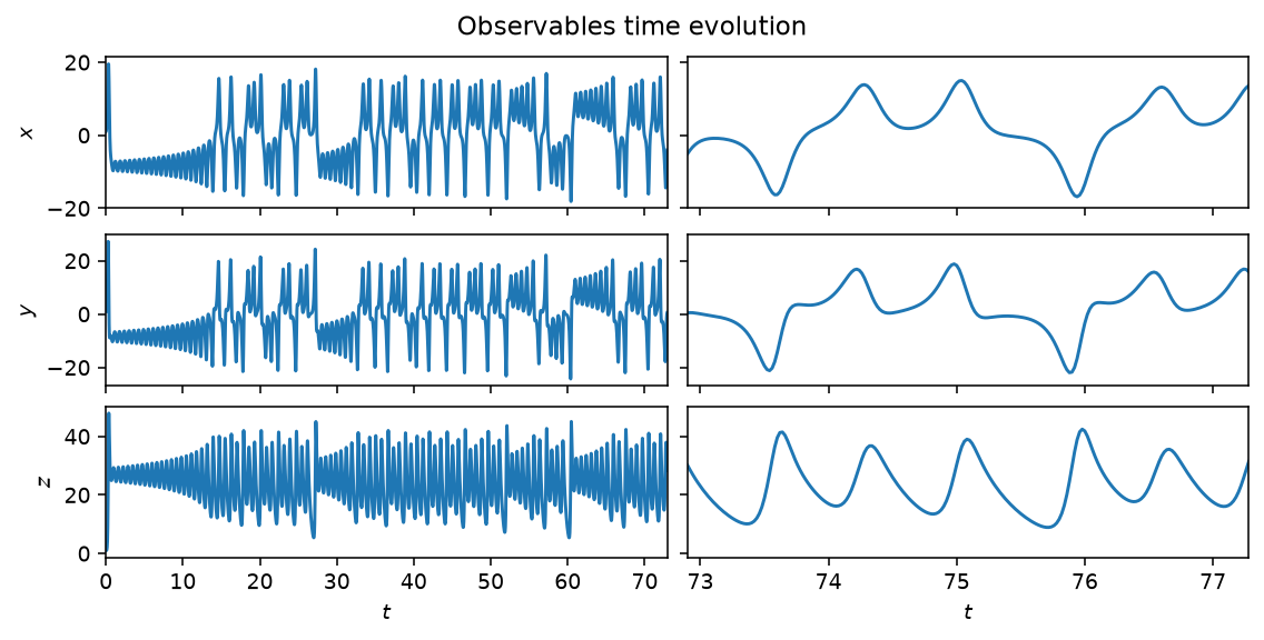
Time evolution of \(x\), \(y\) and \(z\) for \(\rho=28\), past the initial transient. Left: the full run. Right: the last four Lyapunov times, showing the characteristic double-lobe switching of the attractor.

Quickstart

from dynamodels.physical import Lorenz63

model = Lorenz63(rho=28., sigma=10., beta=8./3, dt=0.02)
psi, t = model.time_integrate(Nt=5000)
model.update_history(psi, t)
model.visualize_attractor()   # the classical butterfly, in 3-D and its three projections
model.close()

observe_dims (default [0, 1, 2], all three states) selects which components are observable; Lorenz63(observe_dims=[0]) restricts the model to observing \(x\) alone, as in a partial-observation data-assimilation setup.

Nonlinear diagnostics

Diagnostics from ntsa.characterize, left to right: the observable time series with a zoomed inset; power spectral density; the 3-D delay-embedded portrait; the first-return map of the maxima; a plane-crossing Poincare section; a recurrence plot; a 3-D classical-MDS embedding of the full state; and the Lyapunov spectrum, confirming the chaotic classification.

Reference

Lorenz, E. N. (1963). Deterministic nonperiodic flow. Journal of the Atmospheric Sciences, 20(2), 130-141.

API

dynamodels.physical.lorenz63.Lorenz63

Bases: Model

Lorenz (1963) system — chaotic benchmark with three state variables.

\[ \dot{x} = \sigma (y - x), \qquad \dot{y} = x (\rho - z) - y, \qquad \dot{z} = x y - \beta z. \]

With the classical parameters (\(\sigma = 10\), \(\rho = 28\), \(\beta = 8/3\)) the system is chaotic with leading Lyapunov exponent \(\lambda_1 \approx 0.906\).

References

Lorenz (1963). Deterministic nonperiodic flow. J. Atmos. Sci., 20, 130–141.

Source code in dynamodels/physical/lorenz63.py

class Lorenz63(Model):
    r"""Lorenz (1963) system — chaotic benchmark with three state variables.

    $$
    \dot{x} = \sigma (y - x), \qquad
    \dot{y} = x (\rho - z) - y, \qquad
    \dot{z} = x y - \beta z.
    $$

    With the classical parameters ($\sigma = 10$, $\rho = 28$, $\beta = 8/3$) the
    system is chaotic with leading Lyapunov exponent $\lambda_1 \approx 0.906$.

    References
    ----------
    Lorenz (1963). Deterministic nonperiodic flow. *J. Atmos. Sci.*, 20, 130–141.
    """

    # --- Core Physics Parameters ---
    t_lyap = 0.9056 ** (-1)
    t_transient = 10 * t_lyap
    t_CR = 4 * t_lyap
    Nq = 3

    rho = 28.
    sigma = 10.
    beta = 8. / 3.

    # --- Ensemble/Augmentation Configuration Placeholders (Required by Model Base Class) ---
    # These are populated later, but required for property calculations in Model
    est_a: list[str] = []

    # --- Parameter and State Labels ---
    params = ['rho', 'sigma', 'beta']
    extra_print_params = ['observe_dims', 'Nq', 't_lyap']

    # __________________________ Init method ___________________________ #
    def __init__(self, **model_dict):


        psi0 = model_dict.pop('psi0', np.array([1.0, 1.0, 1.0]))
        dt = model_dict.pop('dt', 0.02)

        self.observe_dims = model_dict.pop('observe_dims', [0, 1, 2]) # Default to observing all dimensions if not specified
        self.Nq = len(self.observe_dims)

        super().__init__(psi0=psi0, dt=dt, integrator_class=IVPIntegrator, **model_dict)

        # measured 1/lambda1 at this rho (set once: params change by re-instantiation)
        self.t_lyap = self.t_lyap_from_table(self.rho, _LAM1_MEASURED, Lorenz63.t_lyap)

        self.alpha_labels = dict(rho='$\\rho$', sigma='$\\sigma$', beta='$\\beta$')


    # _______________ Lorenz63 specific properties and methods ________________ #

    @property
    def obs_labels(self):
        return [self.state_labels[kk] for kk in self.observe_dims]

    @property
    def state_labels(self):
        return ['$x$', '$y$', '$z$']

    def get_observables(self, Nt=1, **kwargs):
        if Nt == 1:
            return self.hist[-1, self.observe_dims, :]
        else:
            return self.hist[-Nt:, self.observe_dims, :]

    @staticmethod
    def time_derivative(t, psi, sigma, rho, beta):
        """
        Calculates the time derivative of the Lorenz 63 system.
        Note: This derivative must handle the augmented state vector (psi).
        The augmented parameters are stored after the core state (x, y, z).
        """

        x1, x2, x3 = psi[:3]

        # The parameter values used for the current derivative calculation
        # These come from the 'params' dict passed by the integrator
        dx1 = sigma * (x2 - x1)
        dx2 = x1 * (rho - x3) - x2
        dx3 = x1 * x2 - beta * x3

        return (dx1, dx2, dx3) + (0,) * (len(psi) - 3)


    def visualize_attractor(self, psi_cases=None, **kwargs):
        """
        Visualizes the Lorenz attractor for given state trajectories.
        Parameters
        ----------
        psi_cases : list, optional
            State trajectories to plot, each of shape ``(Nt, 3)`` or ``(Nt, 3, Ne)``.
            Defaults to the model's own history.
        **kwargs
            Plotting options forwarded to the helper (``color``, ``figsize``, ...).
        """
        if psi_cases is None:
            psi_cases = [self.hist[:, :3, :]]

        plot_attractor(psi_cases, **kwargs)

time_derivative(t, psi, sigma, rho, beta) staticmethod

Calculates the time derivative of the Lorenz 63 system. Note: This derivative must handle the augmented state vector (psi). The augmented parameters are stored after the core state (x, y, z).

Source code in dynamodels/physical/lorenz63.py

@staticmethod
def time_derivative(t, psi, sigma, rho, beta):
    """
    Calculates the time derivative of the Lorenz 63 system.
    Note: This derivative must handle the augmented state vector (psi).
    The augmented parameters are stored after the core state (x, y, z).
    """

    x1, x2, x3 = psi[:3]

    # The parameter values used for the current derivative calculation
    # These come from the 'params' dict passed by the integrator
    dx1 = sigma * (x2 - x1)
    dx2 = x1 * (rho - x3) - x2
    dx3 = x1 * x2 - beta * x3

    return (dx1, dx2, dx3) + (0,) * (len(psi) - 3)

visualize_attractor(psi_cases=None, **kwargs)

Visualizes the Lorenz attractor for given state trajectories.

Parameters:

Name	Type	Description	Default
psi_cases	list	State trajectories to plot, each of shape (Nt, 3) or (Nt, 3, Ne). Defaults to the model's own history.	None
**kwargs		Plotting options forwarded to the helper (color, figsize, ...).	{}

Source code in dynamodels/physical/lorenz63.py

def visualize_attractor(self, psi_cases=None, **kwargs):
    """
    Visualizes the Lorenz attractor for given state trajectories.
    Parameters
    ----------
    psi_cases : list, optional
        State trajectories to plot, each of shape ``(Nt, 3)`` or ``(Nt, 3, Ne)``.
        Defaults to the model's own history.
    **kwargs
        Plotting options forwarded to the helper (``color``, ``figsize``, ...).
    """
    if psi_cases is None:
        psi_cases = [self.hist[:, :3, :]]

    plot_attractor(psi_cases, **kwargs)