Skip to content

Kuramoto-Sivashinsky (2-D)

The two-dimensional, anisotropic extension of the 1-D Kuramoto-Sivashinsky equation adds a second spatial direction with its own hyperviscosity \(\nu_2\),

\[ u_t + \left(u_{xx} + \alpha\, u_{yy}\right) + \nu_1 \left(\partial_x^2 + \alpha\, \partial_y^2\right)^2 u + \tfrac{1}{2}\left(u_x^2 + \alpha\, u_y^2\right) = 0, \qquad (x, y) \in (0, 2\ell]^2, \]

doubly periodic, with anisotropy ratio \(\alpha=\nu_2/\nu_1\). The state is the physical field itself (not its Fourier transform, as in the 1-D case), flattened to shape (Nx * Ny, m). Which regime the equation settles into — periodic, travelling, quasiperiodic, or chaotic — depends on \((\nu_1, \nu_2)\); five named regimes are pre-tabulated in CASES and selected with case='...'. The class defaults are the periodic regime.
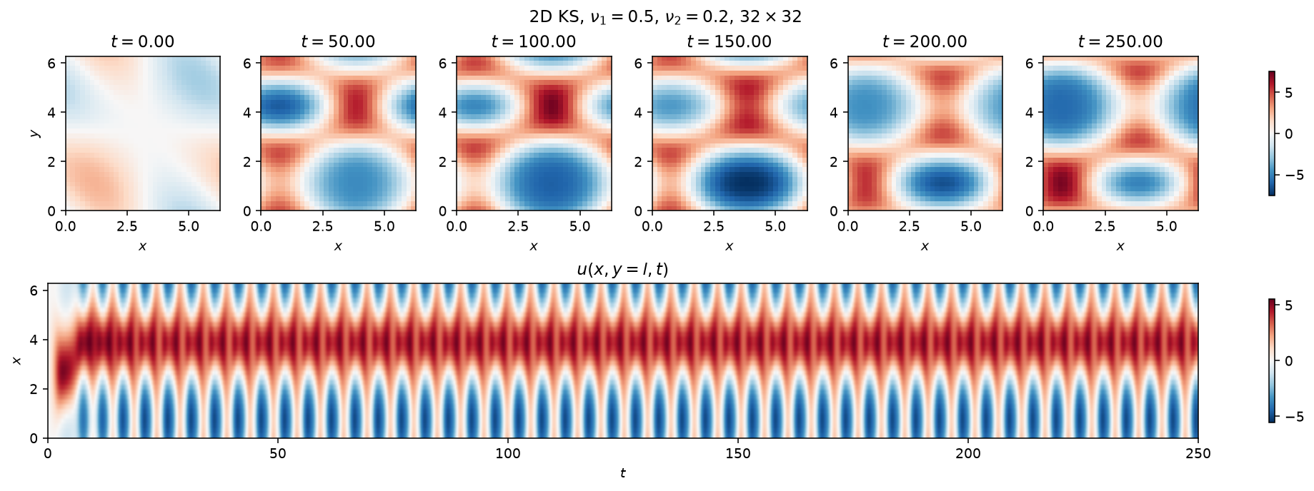
Kuramoto-Sivashinsky 2-D spatiotemporal evolution

Top: six snapshots of the field \(u(x,y,t)\) at \(\nu_1=0.5\), \(\nu_2=0.2\) (the periodic regime), evenly spaced past the transient. Bottom: space-time diagram of the mid-domain slice \(u(x, y=\ell, t)\), showing the pattern travel across the domain and repeat.

A single snapshot, or a 1-D slice's space-time diagram, cannot show how the whole 2-D field evolves. For the chaotic regime, an animation does:
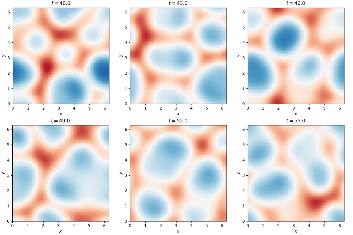
Kuramoto-Sivashinsky 2-D chaotic field, animated

case='chaotic' (\(\nu_1=\nu_2=0.1\), \(64\times64\)): the field \(u(x,y,t)\) past the transient, sampled every few output steps. Structures merge, split and drift with no repeating pattern -- the two-dimensional analogue of the cellular chaos on the 1-D KS page.

Quickstart

from dynamodels.physical import KS2D

model = KS2D()   # class defaults are the periodic regime; try case='chaotic' too
psi, t = model.time_integrate(Nt=4000)
model.update_history(psi, t)
model.visualize_spatiotemporal_hist()
model.close()
Regime \(\nu_1\) \(\nu_2\) Grid \(\mathrm{d}t\)
periodic (default) 0.5 0.2 32x32 0.01
travelling 0.5 0.35 32x32 0.1
quasi-periodic 0.5 0.1 32x32 0.01
chaotic 0.1 0.1 64x64 0.01
chaotic_B 0.3 0.1 64x64 0.01

Explicit keyword arguments override a case's values, e.g. KS2D(case='chaotic', Nx=128, Ny=128).

Nonlinear diagnostics

ntsa characterization of KS2D

Diagnostics from ntsa.characterize on the chaotic case, at a single grid point, left to right: the observable time series with a zoomed inset; power spectral density; the 3-D delay-embedded portrait; the first-return map of the maxima; a plane-crossing Poincare section; a recurrence plot; a 3-D classical-MDS embedding of the full 2-D field; and the leading Lyapunov exponent, estimated Jacobian-free from perturbation growth since KS2D steps with time_step rather than time_derivative.

Reference

Kuramoto, Y., & Tsuzuki, T. (1976). Persistent propagation of concentration waves in dissipative media far from thermal equilibrium. Progress of Theoretical Physics, 55(2), 356-369.

API

dynamodels.physical.kuramoto_sivashinsky_2d.KS2D

Bases: Model

Anisotropic two-dimensional Kuramoto-Sivashinsky equation.

\[ u_t + \left(u_{xx} + \alpha\, u_{yy}\right) + \nu_1 \left(\partial_x^2 + \alpha\, \partial_y^2\right)^2 u + \tfrac{1}{2}\left(u_x^2 + \alpha\, u_y^2\right) = 0, \qquad (x, y) \in (0, 2\ell]^2, \]

doubly periodic, with anisotropy ratio \(\alpha = \nu_2/\nu_1\). Solved pseudo-spectrally (full 2-D FFT) with the ETDRK4 scheme; the exponential coefficients are evaluated by the Kassam-Trefethen contour integral. The zero mode is projected out at every step (the equation only defines \(u\) up to a constant), so the field stays zero-mean.

The state is the PHYSICAL field flattened to shape (Nx*Ny, m) -- real valued, so observables are plain state rows and ensemble filters need no complex-state handling.

Known regimes on the default \(\ell = \pi\) domain (see the qlROM-DA study):

regime nu1 nu2 grid dt t_transient t_CR
periodic 0.5 0.2 32x32 0.01 100. 10.
travelling 0.5 0.35 32x32 0.1 100. 10.
quasi-periodic 0.5 0.1 32x32 0.01 100. 10.
chaotic 0.1 0.1 64x64 0.01 40. 4.
chaotic_B 0.3 0.1 64x64 0.01 100. 10.

The class defaults are the 'periodic' regime; pass case='chaotic' etc. (see CASES) to select another. Explicit kwargs win over the case values, e.g. KS2D(case='chaotic', Nx=128, Ny=128).

Source code in dynamodels/physical/kuramoto_sivashinsky_2d.py
 19
 20
 21
 22
 23
 24
 25
 26
 27
 28
 29
 30
 31
 32
 33
 34
 35
 36
 37
 38
 39
 40
 41
 42
 43
 44
 45
 46
 47
 48
 49
 50
 51
 52
 53
 54
 55
 56
 57
 58
 59
 60
 61
 62
 63
 64
 65
 66
 67
 68
 69
 70
 71
 72
 73
 74
 75
 76
 77
 78
 79
 80
 81
 82
 83
 84
 85
 86
 87
 88
 89
 90
 91
 92
 93
 94
 95
 96
 97
 98
 99
100
101
102
103
104
105
106
107
108
109
110
111
112
113
114
115
116
117
118
119
120
121
122
123
124
125
126
127
128
129
130
131
132
133
134
135
136
137
138
139
140
141
142
143
144
145
146
147
148
149
150
151
152
153
154
155
156
157
158
159
160
161
162
163
164
165
166
167
168
169
170
171
172
173
174
175
176
177
178
179
180
181
182
183
184
185
186
187
188
189
190
191
192
193
194
195
196
197
198
199
200
201
202
203
204
205
206
207
208
209
210
211
212
213
214
215
216
217
218
219
220
221
222
223
224
225
226
227
228
229
230
231
232
233
234
235
236
237
238
239
240
241
242
243
244
245
246
247
248
249
250
251
252
253
254
255
256
257
258
259
260
261
262
263
264
265
266
267
268
269
270
271
272
273
274
275
276
277
278
279
280
281
282
283
284
285
286
287
288
289
290
291
292
293
294
295
296
297
298
299
300
301
302
303
304
305
306
307
308
309
310
311
312
313
314
315
316
317
318
319
320
321
322
323
324
325
326
327
328
329
330
331
332
333
334
335
336
337
338
339
340
341
342
343
344
345
346
347
348
349
350
351
352
353
354
355
356
357
358
359
360
361
362
363
364
365
366
367
368
369
370
371
372
373
374
375
376
377
378
379
380
381
382
383
384
385
386
387
388
389
390
391
392
393
394
395
396
397
398
399
400
class KS2D(Model):

    r"""Anisotropic two-dimensional Kuramoto-Sivashinsky equation.

    $$
    u_t + \left(u_{xx} + \alpha\, u_{yy}\right)
        + \nu_1 \left(\partial_x^2 + \alpha\, \partial_y^2\right)^2 u
        + \tfrac{1}{2}\left(u_x^2 + \alpha\, u_y^2\right) = 0,
    \qquad (x, y) \in (0, 2\ell]^2,
    $$

    doubly periodic, with anisotropy ratio $\alpha = \nu_2/\nu_1$. Solved
    pseudo-spectrally (full 2-D FFT) with the ETDRK4 scheme; the exponential
    coefficients are evaluated by the Kassam-Trefethen contour integral. The
    zero mode is projected out at every step (the equation only defines $u$ up
    to a constant), so the field stays zero-mean.

    The state is the PHYSICAL field flattened to shape (Nx*Ny, m) -- real
    valued, so observables are plain state rows and ensemble filters need no
    complex-state handling.

    Known regimes on the default $\ell = \pi$ domain (see the qlROM-DA study):

    | regime         | nu1 | nu2  | grid  | dt   | t_transient | t_CR |
    |----------------|-----|------|-------|------|-------------|------|
    | periodic       | 0.5 | 0.2  | 32x32 | 0.01 | 100.        | 10.  |
    | travelling     | 0.5 | 0.35 | 32x32 | 0.1  | 100.        | 10.  |
    | quasi-periodic | 0.5 | 0.1  | 32x32 | 0.01 | 100.        | 10.  |
    | chaotic        | 0.1 | 0.1  | 64x64 | 0.01 | 40.        | 4.  |
    | chaotic_B      | 0.3 | 0.1  | 64x64 | 0.01 | 100.        | 10.  |

    The class defaults are the 'periodic' regime; pass ``case='chaotic'`` etc.
    (see `CASES`) to select another. Explicit kwargs win over the case values,
    e.g. ``KS2D(case='chaotic', Nx=128, Ny=128)``.
    """

    t_transient = 100.
    t_CR = 10.

    case = None  # default case; can be overridden in __init__ or by kwargs
    Nq = 4                 # Number of sensors
    Nx = 32                # Grid points in x
    Ny = 32                # Grid points in y
    nu1 = 0.5              # Fourth-order 'viscosity' parameter
    nu2 = 0.2              # Anisotropic counterpart (alpha = nu2 / nu1)
    l = float(np.pi)       # noqa: E741 -- domain half-length (0, 2l]^2, matches the ks2d study notation

    Mcontour = 32          # Contour-integral points for the ETDRK4 coefficients
    Rcontour = 15.0        # Contour radius

    # nu1/nu2 are estimable (per-member ETDRK4 coefficients are rebuilt when a
    # DA analysis moves them); the grid and domain stay structural
    params = ['nu1', 'nu2']
    fixed_params = ['Nx', 'Ny', 'l']
    extra_print_params = ['Nx', 'Ny', 'nu1', 'nu2']
    sensor_placement_method = 'grid'

    def __init__(self, **model_dict):
        """Initialize the 2D KS model.

        Parameters
        ----------
        **model_dict
            Model parameters; supported keys are:

            - ``case`` : str, a named regime from `CASES`; its values are
              defaults that any explicit kwarg below overrides.
            - ``Nx``, ``Ny`` : int, grid points per direction (must be even).
            - ``nu1``, ``nu2`` : float, viscosity parameters (alpha = nu2/nu1).
            - ``l`` : float, domain half-length, domain is (0, 2l]^2.
            - ``dt`` : float, time step size.
            - ``Nq`` : int, number of sensors.
            - ``sensor_placement_method`` : str, ``'grid'`` or ``'random'``.
            - ``seed`` : int, random seed for sensor placement.
            - ``psi0`` : ndarray, initial PHYSICAL field, shape (Nx*Ny,) or
              (Nx*Ny, m) (optional; defaults to sin(X+Y) + sin(X) + sin(Y)).
        """
        self.case = model_dict.pop('case', None)
        if self.case is not None:
            if self.case not in CASES:
                raise ValueError(f"Unknown case '{self.case}'. Must be one of {list(CASES)}.")
            for key, val in CASES[self.case].items():
                model_dict.setdefault(key, val)  # explicit kwargs win over the case

        for key in list(model_dict.keys()):
            if key in vars(KS2D):
                setattr(self, key, model_dict.pop(key))

        if self.Nx % 2 != 0 or self.Ny % 2 != 0:
            raise ValueError("Nx and Ny must be even.")
        if self.nu1 <= 0 or self.nu2 <= 0:
            raise ValueError("nu1 and nu2 must be positive.")

        # Physical grid on (0, 2l]^2
        self.dx = 2.0 * self.l / self.Nx
        self.dy = 2.0 * self.l / self.Ny
        self.X, self.Y = np.meshgrid(self.x, self.y, indexing='ij')

        # Full FFT wavenumbers (positive Nyquist convention)
        dk = np.pi / self.l
        kx = np.concatenate((np.arange(0, self.Nx // 2 + 1),
                             np.arange(-self.Nx // 2 + 1, 0))) * dk
        ky = np.concatenate((np.arange(0, self.Ny // 2 + 1),
                             np.arange(-self.Ny // 2 + 1, 0))) * dk
        self.kX, self.kY = np.meshgrid(kx, ky, indexing='ij')

        self.aniso = self.nu2 / self.nu1     # alpha in the equation; Model reserves .alpha
        self.Lhat = self._lhat(self.nu1, self.nu2)

        self._etdrk4_cache = None
        self._member_terms = None

        #  Select sensors ___________________________ #
        if self.sensor_placement_method == 'grid':
            self.sensor_locations = np.linspace(0, self.Nx * self.Ny - 1, self.Nq,
                                                endpoint=True, dtype=int)
        elif self.sensor_placement_method == 'random':
            self.sensor_locations = self.rng.integers(0, self.Nx * self.Ny - 1, self.Nq)
        else:
            raise NotImplementedError(f"sensor_placement_method "
                                      f"'{self.sensor_placement_method}' not recognized.")

        #   Init Model  #
        dt = model_dict.pop('dt', 0.01)
        psi0 = model_dict.pop('psi0', None)
        if psi0 is None:
            u0 = np.sin(self.X + self.Y) + np.sin(self.X) + np.sin(self.Y)
            u0 -= np.mean(u0)
            psi0 = u0.reshape(-1, 1)

        super().__init__(psi0=psi0, dt=dt, integrator_class=DiscreteIntegrator, **model_dict)

        self.alpha_labels = dict(nu1='$\\nu_1$', nu2='$\\nu_2$')
        self.alpha_lims = dict(nu1=(0.01, 1.0), nu2=(0.01, 1.0))

    # _______________ Modified Model methods ________________ #

    @property
    def obs_labels(self):
        return [f"$u(\\mathbf{{x}}_{{{j+1}}})$" for j in np.arange(self.Nq)]

    @property
    def state_labels(self):
        return [f"$u_{{{j+1}}}$" for j in np.arange(self.Nphi)]

    def get_observables(self, Nt=1, loc=None, **kwargs):
        """Observable state at the sensor locations (the state is already the
        physical field, so observables are plain rows of the flattened state).

        Parameters
        ----------
        Nt : int
            Number of time steps to retrieve. Default is 1.
        loc : array-like or str, optional
            Flattened-grid sensor indices; 'all' returns the whole field;
            None (default) uses the model's sensor locations.
        """
        if loc is None:
            loc = self.sensor_locations
        elif isinstance(loc, str) and loc.lower() == 'all':
            loc = np.arange(self.Nx * self.Ny)
        elif isinstance(loc, str):
            raise ValueError("loc must be None, 'all', or array-like integer indices.")

        loc = np.asarray(loc, dtype=int)

        if Nt == 1:
            return self.hist[-1, loc]
        else:
            return self.hist[-Nt:, loc]

    # _______________ KS2D specific properties and methods ________________ #

    @property
    def x(self):
        return np.arange(self.Nx) * self.dx

    @property
    def y(self):
        return np.arange(self.Ny) * self.dy

    def _lhat(self, nu1, nu2):
        """Diagonal spectral operator for given nu values. Scalars give the
        shared (Nx, Ny) operator; per-member arrays of length m give a
        (Nx, Ny, m) stack."""
        nu1, nu2 = np.asarray(nu1, dtype=float), np.asarray(nu2, dtype=float)
        kX, kY = (self.kX, self.kY) if nu1.ndim == 0 else (self.kX[:, :, None], self.kY[:, :, None])
        a = nu2 / nu1
        return (kX**2 + a * kY**2
                - nu1 * (kX**4 + 2.0 * a * kX**2 * kY**2 + a**2 * kY**4))

    @property
    def ETDRK4_f_terms(self):
        """ETDRK4 coefficient arrays (Nx, Ny) for the constructed (nu1, nu2),
        recomputed if dt changed."""
        if self._etdrk4_cache is None or self._etdrk4_cache[0] != self.dt:
            self._etdrk4_cache = (self.dt, self._compute_etdrk4_terms())
        return self._etdrk4_cache[1]

    def _compute_etdrk4_terms(self, Lhat=None):
        """Kassam-Trefethen contour-integral evaluation of the ETDRK4
        coefficients for the diagonal spectral operator `Lhat` (defaults to
        the constructed one; a (Nx, Ny, m) stack gives per-member terms)."""
        if Lhat is None:
            Lhat = self.Lhat
        mm = np.arange(1, self.Mcontour + 1)
        r = self.Rcontour * np.exp(1j * np.pi * (mm - 0.5) / self.Mcontour)
        LR = self.dt * Lhat[..., None] + r

        with np.errstate(divide='ignore', invalid='ignore', over='ignore'):
            terms = dict(
                E=np.exp(self.dt * Lhat),
                E2=np.exp(0.5 * self.dt * Lhat),
                Q=self.dt * np.real(np.mean((np.exp(LR / 2.0) - 1.0) / LR, axis=-1)),
                f1=self.dt * np.real(np.mean(
                    (-4.0 - LR + np.exp(LR) * (4.0 - 3.0 * LR + LR**2)) / LR**3, axis=-1)),
                f2=self.dt * np.real(np.mean(
                    (2.0 + LR + np.exp(LR) * (-2.0 + LR)) / LR**3, axis=-1)),
                f3=self.dt * np.real(np.mean(
                    (-4.0 - 3.0 * LR - LR**2 + np.exp(LR) * (4.0 - LR)) / LR**3, axis=-1)),
            )
        return terms

    def _terms_for(self, alpha):
        """ETDRK4 terms (plus per-member anisotropy) for a list of per-member
        alpha dicts; falls through to the shared terms when every member sits
        at the constructed (nu1, nu2)."""
        nu1 = np.array([a['nu1'] for a in alpha], dtype=float)
        nu2 = np.array([a['nu2'] for a in alpha], dtype=float)
        if np.all(nu1 == self.nu1) and np.all(nu2 == self.nu2):
            return self.ETDRK4_f_terms
        key = (self.dt, nu1.tobytes(), nu2.tobytes())
        if self._member_terms is None or self._member_terms[0] != key:
            # ponytail: full contour rebuild whenever the nus move -- cheap next
            # to stepping, and only a DA analysis (or a new alpha) moves them
            terms = self._compute_etdrk4_terms(self._lhat(nu1, nu2))
            terms['aniso'] = nu2 / nu1
            self._member_terms = (key, terms)
        return self._member_terms[1]

    def _nonlinear_hat(self, vhat, aniso=None):
        """N(u) = -1/2 F[u_x^2 + alpha u_y^2] for spectral fields (Nx, Ny, m);
        `aniso` may be scalar or per-member (m,)."""
        if aniso is None:
            aniso = self.aniso
        vx = np.fft.ifft2(1j * self.kX[:, :, None] * vhat, axes=(0, 1)).real
        vy = np.fft.ifft2(1j * self.kY[:, :, None] * vhat, axes=(0, 1)).real
        return -0.5 * np.fft.fft2(vx * vx + aniso * vy * vy, axes=(0, 1))

    def ETDRK4_step(self, u, terms=None):
        """One ETDRK4 step of physical fields u with shape (Nx, Ny, m).
        `terms` defaults to the shared coefficients; per-member (Nx, Ny, m)
        stacks from `_terms_for` are used as-is."""
        c = self.ETDRK4_f_terms if terms is None else terms
        E, E2, Q, f1, f2, f3 = (c[k][:, :, None] if c[k].ndim == 2 else c[k]
                                for k in ('E', 'E2', 'Q', 'f1', 'f2', 'f3'))
        aniso = c.get('aniso', self.aniso)

        u = u - np.mean(u, axis=(0, 1), keepdims=True)
        vhat = np.fft.fft2(u, axes=(0, 1))

        Nv = self._nonlinear_hat(vhat, aniso)
        a = E2 * vhat + Q * Nv
        Na = self._nonlinear_hat(a, aniso)
        b = E2 * vhat + Q * Na
        Nb = self._nonlinear_hat(b, aniso)
        cstage = E2 * a + Q * (2.0 * Nb - Nv)
        Nc = self._nonlinear_hat(cstage, aniso)

        vhat_next = E * vhat + f1 * Nv + 2.0 * f2 * (Na + Nb) + f3 * Nc
        u_next = np.fft.ifft2(vhat_next, axes=(0, 1)).real
        return u_next - np.mean(u_next, axis=(0, 1), keepdims=True)

    def time_step(self, Nt=10, averaged=False, alpha=None):
        """Advance all m members Nt ETDRK4 steps.

        Parameters
        ----------
        alpha : list of dict, optional
            Per-member parameter dicts (as from `get_alpha`); defaults to the
            values carried in the (possibly augmented) current state. Members
            with nus away from the constructed ones get their own ETDRK4
            coefficients.

        Returns
        -------
        psi : np.ndarray
            Trajectory of shape (Nt + 1, Nphi [+ Na], m), including the
            current state; estimated-parameter rows are carried unchanged.
        t : np.ndarray
            Time points, shape (Nt + 1,).
        """
        psi0 = self.current_state
        if psi0.ndim == 1:
            psi0 = psi0[:, None]
        m = psi0.shape[1]
        Nu = self.Nx * self.Ny
        u0, aug = psi0[:Nu], psi0[Nu:]   # estimated-parameter rows ride along unchanged

        if alpha is None:
            alpha = self.get_alpha(psi0)

        t = np.round(self.current_time + np.arange(Nt + 1) * self.dt, self.precision_t)

        if averaged and m > 1:
            mean_alpha = [{k: float(np.mean([a[k] for a in alpha])) for k in self.params}]
            terms = self._terms_for(mean_alpha)
            u_mean = np.mean(u0, axis=1, keepdims=True)
            deviation = u0 - u_mean
            u = u_mean.reshape(self.Nx, self.Ny, 1)
            frames = [u]
            for _ in range(Nt):
                frames.append(self.ETDRK4_step(frames[-1], terms))
            psi = np.stack([f.reshape(-1, 1) + deviation for f in frames], axis=0)
        else:
            terms = self._terms_for(alpha)
            u = u0.reshape(self.Nx, self.Ny, m)
            frames = [u]
            for _ in range(Nt):
                frames.append(self.ETDRK4_step(frames[-1], terms))
            psi = np.stack([f.reshape(-1, m) for f in frames], axis=0)

        if aug.shape[0]:
            psi = np.concatenate([psi, np.broadcast_to(aug, (Nt + 1, *aug.shape))], axis=1)
        return psi, t

    def get_energy(self, Nt=0, u=None):
        """Spatially averaged L2 energy, E = mean(u^2), shape (Nt, m)."""
        if u is None:
            u = self.get_observable_hist(Nt=Nt, loc='all')
        if u.ndim == 2:
            u = u[np.newaxis, :]
        assert u.shape[1] == self.Nx * self.Ny
        return np.mean(u**2, axis=1)

    def get_enstrophy(self, Nt=0, u=None):
        """Spatially averaged enstrophy, mean(u_x^2 + alpha u_y^2), shape (Nt, m)."""
        if u is None:
            u = self.get_observable_hist(Nt=Nt, loc='all')
        if u.ndim == 2:
            u = u[np.newaxis, :]
        Nt_, _, m = u.shape
        vhat = np.fft.fft2(u.reshape(Nt_, self.Nx, self.Ny, m), axes=(1, 2))
        ux = np.fft.ifft2(1j * self.kX[None, :, :, None] * vhat, axes=(1, 2)).real
        uy = np.fft.ifft2(1j * self.kY[None, :, :, None] * vhat, axes=(1, 2)).real
        return np.mean((ux**2 + self.aniso * uy**2).reshape(Nt_, -1, m), axis=1)

    def visualize_spatiotemporal_hist(self,
                                      nframes=6, member=0, **kwargs):
        """Snapshot strip of the physical field u(x, y) for one ensemble member,
        plus a space-time diagram of the mid-domain slice u(x, y = l, t)."""
        u_hist = self.get_observable_hist(loc='all')
        t = self.hist_t
        u = u_hist[:, :, member].reshape(len(t), self.Nx, self.Ny)
        idx = np.linspace(0, len(t) - 1, nframes, dtype=int)
        lim = np.max(np.abs(u[idx]))

        fig = plt.figure(figsize=(2.2 * nframes, 4.8), constrained_layout=True)
        gs = fig.add_gridspec(2, nframes)
        axs = [fig.add_subplot(gs[0, jj]) for jj in range(nframes)]
        im = None
        for ax, ii in zip(axs, idx):
            im = ax.imshow(u[ii].T,
                           origin='lower', cmap='RdBu_r', vmin=-lim, vmax=lim,
                           extent=(0, 2 * self.l, 0, 2 * self.l))
            ax.set(title=f"$t={t[ii]:.2f}$", xlabel="$x$")
        axs[0].set(ylabel="$y$")
        assert im is not None
        fig.colorbar(im, ax=axs, shrink=0.8)

        # space-time diagram along the mid-domain slice y = l
        u_slice = u[:, :, self.Ny // 2]
        ax_st = fig.add_subplot(gs[1, :])
        lim_st = np.max(np.abs(u_slice))
        im_st = ax_st.imshow(u_slice.T, aspect='auto', origin='lower',
                             cmap='RdBu_r', vmin=-lim_st, vmax=lim_st,
                             extent=(t[0], t[-1], 0, 2 * self.l))
        ax_st.set(xlabel="$t$", ylabel="$x$", title=r"$u(x, y = l, t)$")
        fig.colorbar(im_st, ax=ax_st, shrink=0.8)

        fig.suptitle(rf"2D KS, $\nu_1={self.nu1}$, $\nu_2={self.nu2}$, "
                     rf"${self.Nx}\times{self.Ny}$")

ETDRK4_f_terms property

ETDRK4 coefficient arrays (Nx, Ny) for the constructed (nu1, nu2), recomputed if dt changed.

__init__(**model_dict)

Initialize the 2D KS model.

Parameters:

Name Type Description Default
**model_dict

Model parameters; supported keys are:

  • case : str, a named regime from CASES; its values are defaults that any explicit kwarg below overrides.
  • Nx, Ny : int, grid points per direction (must be even).
  • nu1, nu2 : float, viscosity parameters (alpha = nu2/nu1).
  • l : float, domain half-length, domain is (0, 2l]^2.
  • dt : float, time step size.
  • Nq : int, number of sensors.
  • sensor_placement_method : str, 'grid' or 'random'.
  • seed : int, random seed for sensor placement.
  • psi0 : ndarray, initial PHYSICAL field, shape (NxNy,) or (NxNy, m) (optional; defaults to sin(X+Y) + sin(X) + sin(Y)).
{}
Source code in dynamodels/physical/kuramoto_sivashinsky_2d.py
 76
 77
 78
 79
 80
 81
 82
 83
 84
 85
 86
 87
 88
 89
 90
 91
 92
 93
 94
 95
 96
 97
 98
 99
100
101
102
103
104
105
106
107
108
109
110
111
112
113
114
115
116
117
118
119
120
121
122
123
124
125
126
127
128
129
130
131
132
133
134
135
136
137
138
139
140
141
142
143
144
145
146
147
148
149
150
151
152
def __init__(self, **model_dict):
    """Initialize the 2D KS model.

    Parameters
    ----------
    **model_dict
        Model parameters; supported keys are:

        - ``case`` : str, a named regime from `CASES`; its values are
          defaults that any explicit kwarg below overrides.
        - ``Nx``, ``Ny`` : int, grid points per direction (must be even).
        - ``nu1``, ``nu2`` : float, viscosity parameters (alpha = nu2/nu1).
        - ``l`` : float, domain half-length, domain is (0, 2l]^2.
        - ``dt`` : float, time step size.
        - ``Nq`` : int, number of sensors.
        - ``sensor_placement_method`` : str, ``'grid'`` or ``'random'``.
        - ``seed`` : int, random seed for sensor placement.
        - ``psi0`` : ndarray, initial PHYSICAL field, shape (Nx*Ny,) or
          (Nx*Ny, m) (optional; defaults to sin(X+Y) + sin(X) + sin(Y)).
    """
    self.case = model_dict.pop('case', None)
    if self.case is not None:
        if self.case not in CASES:
            raise ValueError(f"Unknown case '{self.case}'. Must be one of {list(CASES)}.")
        for key, val in CASES[self.case].items():
            model_dict.setdefault(key, val)  # explicit kwargs win over the case

    for key in list(model_dict.keys()):
        if key in vars(KS2D):
            setattr(self, key, model_dict.pop(key))

    if self.Nx % 2 != 0 or self.Ny % 2 != 0:
        raise ValueError("Nx and Ny must be even.")
    if self.nu1 <= 0 or self.nu2 <= 0:
        raise ValueError("nu1 and nu2 must be positive.")

    # Physical grid on (0, 2l]^2
    self.dx = 2.0 * self.l / self.Nx
    self.dy = 2.0 * self.l / self.Ny
    self.X, self.Y = np.meshgrid(self.x, self.y, indexing='ij')

    # Full FFT wavenumbers (positive Nyquist convention)
    dk = np.pi / self.l
    kx = np.concatenate((np.arange(0, self.Nx // 2 + 1),
                         np.arange(-self.Nx // 2 + 1, 0))) * dk
    ky = np.concatenate((np.arange(0, self.Ny // 2 + 1),
                         np.arange(-self.Ny // 2 + 1, 0))) * dk
    self.kX, self.kY = np.meshgrid(kx, ky, indexing='ij')

    self.aniso = self.nu2 / self.nu1     # alpha in the equation; Model reserves .alpha
    self.Lhat = self._lhat(self.nu1, self.nu2)

    self._etdrk4_cache = None
    self._member_terms = None

    #  Select sensors ___________________________ #
    if self.sensor_placement_method == 'grid':
        self.sensor_locations = np.linspace(0, self.Nx * self.Ny - 1, self.Nq,
                                            endpoint=True, dtype=int)
    elif self.sensor_placement_method == 'random':
        self.sensor_locations = self.rng.integers(0, self.Nx * self.Ny - 1, self.Nq)
    else:
        raise NotImplementedError(f"sensor_placement_method "
                                  f"'{self.sensor_placement_method}' not recognized.")

    #   Init Model  #
    dt = model_dict.pop('dt', 0.01)
    psi0 = model_dict.pop('psi0', None)
    if psi0 is None:
        u0 = np.sin(self.X + self.Y) + np.sin(self.X) + np.sin(self.Y)
        u0 -= np.mean(u0)
        psi0 = u0.reshape(-1, 1)

    super().__init__(psi0=psi0, dt=dt, integrator_class=DiscreteIntegrator, **model_dict)

    self.alpha_labels = dict(nu1='$\\nu_1$', nu2='$\\nu_2$')
    self.alpha_lims = dict(nu1=(0.01, 1.0), nu2=(0.01, 1.0))

get_observables(Nt=1, loc=None, **kwargs)

Observable state at the sensor locations (the state is already the physical field, so observables are plain rows of the flattened state).

Parameters:

Name Type Description Default
Nt int

Number of time steps to retrieve. Default is 1.

1
loc array - like or str

Flattened-grid sensor indices; 'all' returns the whole field; None (default) uses the model's sensor locations.

None
Source code in dynamodels/physical/kuramoto_sivashinsky_2d.py
164
165
166
167
168
169
170
171
172
173
174
175
176
177
178
179
180
181
182
183
184
185
186
187
188
def get_observables(self, Nt=1, loc=None, **kwargs):
    """Observable state at the sensor locations (the state is already the
    physical field, so observables are plain rows of the flattened state).

    Parameters
    ----------
    Nt : int
        Number of time steps to retrieve. Default is 1.
    loc : array-like or str, optional
        Flattened-grid sensor indices; 'all' returns the whole field;
        None (default) uses the model's sensor locations.
    """
    if loc is None:
        loc = self.sensor_locations
    elif isinstance(loc, str) and loc.lower() == 'all':
        loc = np.arange(self.Nx * self.Ny)
    elif isinstance(loc, str):
        raise ValueError("loc must be None, 'all', or array-like integer indices.")

    loc = np.asarray(loc, dtype=int)

    if Nt == 1:
        return self.hist[-1, loc]
    else:
        return self.hist[-Nt:, loc]

ETDRK4_step(u, terms=None)

One ETDRK4 step of physical fields u with shape (Nx, Ny, m). terms defaults to the shared coefficients; per-member (Nx, Ny, m) stacks from _terms_for are used as-is.

Source code in dynamodels/physical/kuramoto_sivashinsky_2d.py
268
269
270
271
272
273
274
275
276
277
278
279
280
281
282
283
284
285
286
287
288
289
290
def ETDRK4_step(self, u, terms=None):
    """One ETDRK4 step of physical fields u with shape (Nx, Ny, m).
    `terms` defaults to the shared coefficients; per-member (Nx, Ny, m)
    stacks from `_terms_for` are used as-is."""
    c = self.ETDRK4_f_terms if terms is None else terms
    E, E2, Q, f1, f2, f3 = (c[k][:, :, None] if c[k].ndim == 2 else c[k]
                            for k in ('E', 'E2', 'Q', 'f1', 'f2', 'f3'))
    aniso = c.get('aniso', self.aniso)

    u = u - np.mean(u, axis=(0, 1), keepdims=True)
    vhat = np.fft.fft2(u, axes=(0, 1))

    Nv = self._nonlinear_hat(vhat, aniso)
    a = E2 * vhat + Q * Nv
    Na = self._nonlinear_hat(a, aniso)
    b = E2 * vhat + Q * Na
    Nb = self._nonlinear_hat(b, aniso)
    cstage = E2 * a + Q * (2.0 * Nb - Nv)
    Nc = self._nonlinear_hat(cstage, aniso)

    vhat_next = E * vhat + f1 * Nv + 2.0 * f2 * (Na + Nb) + f3 * Nc
    u_next = np.fft.ifft2(vhat_next, axes=(0, 1)).real
    return u_next - np.mean(u_next, axis=(0, 1), keepdims=True)

time_step(Nt=10, averaged=False, alpha=None)

Advance all m members Nt ETDRK4 steps.

Parameters:

Name Type Description Default
alpha list of dict

Per-member parameter dicts (as from get_alpha); defaults to the values carried in the (possibly augmented) current state. Members with nus away from the constructed ones get their own ETDRK4 coefficients.

None

Returns:

Name Type Description
psi ndarray

Trajectory of shape (Nt + 1, Nphi [+ Na], m), including the current state; estimated-parameter rows are carried unchanged.

t ndarray

Time points, shape (Nt + 1,).

Source code in dynamodels/physical/kuramoto_sivashinsky_2d.py
292
293
294
295
296
297
298
299
300
301
302
303
304
305
306
307
308
309
310
311
312
313
314
315
316
317
318
319
320
321
322
323
324
325
326
327
328
329
330
331
332
333
334
335
336
337
338
339
340
341
342
343
def time_step(self, Nt=10, averaged=False, alpha=None):
    """Advance all m members Nt ETDRK4 steps.

    Parameters
    ----------
    alpha : list of dict, optional
        Per-member parameter dicts (as from `get_alpha`); defaults to the
        values carried in the (possibly augmented) current state. Members
        with nus away from the constructed ones get their own ETDRK4
        coefficients.

    Returns
    -------
    psi : np.ndarray
        Trajectory of shape (Nt + 1, Nphi [+ Na], m), including the
        current state; estimated-parameter rows are carried unchanged.
    t : np.ndarray
        Time points, shape (Nt + 1,).
    """
    psi0 = self.current_state
    if psi0.ndim == 1:
        psi0 = psi0[:, None]
    m = psi0.shape[1]
    Nu = self.Nx * self.Ny
    u0, aug = psi0[:Nu], psi0[Nu:]   # estimated-parameter rows ride along unchanged

    if alpha is None:
        alpha = self.get_alpha(psi0)

    t = np.round(self.current_time + np.arange(Nt + 1) * self.dt, self.precision_t)

    if averaged and m > 1:
        mean_alpha = [{k: float(np.mean([a[k] for a in alpha])) for k in self.params}]
        terms = self._terms_for(mean_alpha)
        u_mean = np.mean(u0, axis=1, keepdims=True)
        deviation = u0 - u_mean
        u = u_mean.reshape(self.Nx, self.Ny, 1)
        frames = [u]
        for _ in range(Nt):
            frames.append(self.ETDRK4_step(frames[-1], terms))
        psi = np.stack([f.reshape(-1, 1) + deviation for f in frames], axis=0)
    else:
        terms = self._terms_for(alpha)
        u = u0.reshape(self.Nx, self.Ny, m)
        frames = [u]
        for _ in range(Nt):
            frames.append(self.ETDRK4_step(frames[-1], terms))
        psi = np.stack([f.reshape(-1, m) for f in frames], axis=0)

    if aug.shape[0]:
        psi = np.concatenate([psi, np.broadcast_to(aug, (Nt + 1, *aug.shape))], axis=1)
    return psi, t

get_energy(Nt=0, u=None)

Spatially averaged L2 energy, E = mean(u^2), shape (Nt, m).

Source code in dynamodels/physical/kuramoto_sivashinsky_2d.py
345
346
347
348
349
350
351
352
def get_energy(self, Nt=0, u=None):
    """Spatially averaged L2 energy, E = mean(u^2), shape (Nt, m)."""
    if u is None:
        u = self.get_observable_hist(Nt=Nt, loc='all')
    if u.ndim == 2:
        u = u[np.newaxis, :]
    assert u.shape[1] == self.Nx * self.Ny
    return np.mean(u**2, axis=1)

get_enstrophy(Nt=0, u=None)

Spatially averaged enstrophy, mean(u_x^2 + alpha u_y^2), shape (Nt, m).

Source code in dynamodels/physical/kuramoto_sivashinsky_2d.py
354
355
356
357
358
359
360
361
362
363
364
def get_enstrophy(self, Nt=0, u=None):
    """Spatially averaged enstrophy, mean(u_x^2 + alpha u_y^2), shape (Nt, m)."""
    if u is None:
        u = self.get_observable_hist(Nt=Nt, loc='all')
    if u.ndim == 2:
        u = u[np.newaxis, :]
    Nt_, _, m = u.shape
    vhat = np.fft.fft2(u.reshape(Nt_, self.Nx, self.Ny, m), axes=(1, 2))
    ux = np.fft.ifft2(1j * self.kX[None, :, :, None] * vhat, axes=(1, 2)).real
    uy = np.fft.ifft2(1j * self.kY[None, :, :, None] * vhat, axes=(1, 2)).real
    return np.mean((ux**2 + self.aniso * uy**2).reshape(Nt_, -1, m), axis=1)

visualize_spatiotemporal_hist(nframes=6, member=0, **kwargs)

Snapshot strip of the physical field u(x, y) for one ensemble member, plus a space-time diagram of the mid-domain slice u(x, y = l, t).

Source code in dynamodels/physical/kuramoto_sivashinsky_2d.py
366
367
368
369
370
371
372
373
374
375
376
377
378
379
380
381
382
383
384
385
386
387
388
389
390
391
392
393
394
395
396
397
398
399
400
def visualize_spatiotemporal_hist(self,
                                  nframes=6, member=0, **kwargs):
    """Snapshot strip of the physical field u(x, y) for one ensemble member,
    plus a space-time diagram of the mid-domain slice u(x, y = l, t)."""
    u_hist = self.get_observable_hist(loc='all')
    t = self.hist_t
    u = u_hist[:, :, member].reshape(len(t), self.Nx, self.Ny)
    idx = np.linspace(0, len(t) - 1, nframes, dtype=int)
    lim = np.max(np.abs(u[idx]))

    fig = plt.figure(figsize=(2.2 * nframes, 4.8), constrained_layout=True)
    gs = fig.add_gridspec(2, nframes)
    axs = [fig.add_subplot(gs[0, jj]) for jj in range(nframes)]
    im = None
    for ax, ii in zip(axs, idx):
        im = ax.imshow(u[ii].T,
                       origin='lower', cmap='RdBu_r', vmin=-lim, vmax=lim,
                       extent=(0, 2 * self.l, 0, 2 * self.l))
        ax.set(title=f"$t={t[ii]:.2f}$", xlabel="$x$")
    axs[0].set(ylabel="$y$")
    assert im is not None
    fig.colorbar(im, ax=axs, shrink=0.8)

    # space-time diagram along the mid-domain slice y = l
    u_slice = u[:, :, self.Ny // 2]
    ax_st = fig.add_subplot(gs[1, :])
    lim_st = np.max(np.abs(u_slice))
    im_st = ax_st.imshow(u_slice.T, aspect='auto', origin='lower',
                         cmap='RdBu_r', vmin=-lim_st, vmax=lim_st,
                         extent=(t[0], t[-1], 0, 2 * self.l))
    ax_st.set(xlabel="$t$", ylabel="$x$", title=r"$u(x, y = l, t)$")
    fig.colorbar(im_st, ax=ax_st, shrink=0.8)

    fig.suptitle(rf"2D KS, $\nu_1={self.nu1}$, $\nu_2={self.nu2}$, "
                 rf"${self.Nx}\times{self.Ny}$")