Kuznetsov oscillator

The Kuznetsov oscillator is a simple autonomous generator of quasiperiodic motion: a three-dimensional system that produces periodic, quasiperiodic and chaotic behaviour depending on \((\lambda, \omega_0, \mu)\),

\[ \dot{x} = y, \qquad \dot{y} = y \left( \lambda + z + x^2 - \tfrac{1}{2} x^4 \right) - \omega_0^2 x, \qquad \dot{z} = \mu - x^2. \]

Unlike the Lorenz63 system, which is chaotic at its classical parameters, the Kuznetsov oscillator's class defaults (\(\lambda=0\), \(\omega_0=2\pi\), \(\mu=1\)) sit on a two-frequency quasiperiodic torus, which makes it a useful counter-example when testing whether a chaos-classification method (positive Lyapunov exponent, broadband spectrum) correctly abstains on a non-chaotic attractor.

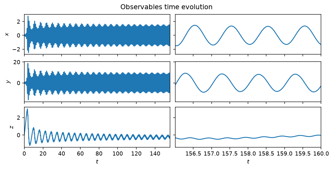
Time evolution of \(x\), \(y\) and \(z\) at the class defaults, past the initial transient. Left: the full run, settling onto the quasiperiodic torus. Right: the last four characteristic times, showing the faster of the two incommensurate frequencies.

Quickstart

from dynamodels.physical import Kuznetsov

model = Kuznetsov(lam=0., omega0=2 * 3.14159, mu=1., dt=0.01)
psi, t = model.time_integrate(Nt=16000)
model.update_history(psi, t)
model.visualize_observable_hist()
model.close()

Nonlinear diagnostics

Diagnostics from ntsa.characterize, left to right: the observable time series with a zoomed inset; power spectral density, with two incommensurate peaks; the 3-D delay-embedded portrait, a torus rather than a fractal attractor; the first-return map and Poincare section, closed curves rather than point clouds; a recurrence plot; a 3-D classical-MDS embedding; and a near-zero leading Lyapunov exponent — quasiperiodic, not chaotic, despite the broadband-looking time series.

Reference

Kuznetsov, A. P., Kuznetsov, S. P., & Stankevich, N. V. (2010). A simple autonomous quasiperiodic self-oscillator. Communications in Nonlinear Science and Numerical Simulation, 15(6), 1676-1681. doi:10.1016/j.cnsns.2009.06.027

API

dynamodels.physical.kuznetsov.Kuznetsov

Bases: Model

Kuznetsov oscillator — autonomous generator of quasiperiodic oscillations.

Three-dimensional system displaying periodic, quasiperiodic and chaotic behaviour as a function of the parameters \([\lambda, \omega_0, \mu]\):

\[ \dot{x} = y, \qquad \dot{y} = y \left( \lambda + z + x^2 - \tfrac{1}{2} x^4 \right) - \omega_0^2 x, \qquad \dot{z} = \mu - x^2. \]

With the default parameters (\(\lambda = 0\), \(\omega_0 = 2\pi\), \(\mu = 1\)) the attractor is a two-frequency quasiperiodic torus.

References

Kuznetsov, Kuznetsov & Stankevich (2010). A simple autonomous quasiperiodic self-oscillator. Commun. Nonlinear Sci. Numer. Simul., 15, 1676–1681. DOI: 10.1016/j.cnsns.2009.06.027.

Source code in dynamodels/physical/kuznetsov.py

class Kuznetsov(Model):
    r"""Kuznetsov oscillator — autonomous generator of quasiperiodic oscillations.

    Three-dimensional system displaying periodic, quasiperiodic and chaotic
    behaviour as a function of the parameters $[\lambda, \omega_0, \mu]$:

    $$
    \dot{x} = y, \qquad
    \dot{y} = y \left( \lambda + z + x^2 - \tfrac{1}{2} x^4 \right) - \omega_0^2 x, \qquad
    \dot{z} = \mu - x^2.
    $$

    With the default parameters ($\lambda = 0$, $\omega_0 = 2\pi$, $\mu = 1$)
    the attractor is a two-frequency quasiperiodic torus.

    References
    ----------
    Kuznetsov, Kuznetsov & Stankevich (2010). A simple autonomous quasiperiodic
    self-oscillator. *Commun. Nonlinear Sci. Numer. Simul.*, 15, 1676–1681.
    [DOI: 10.1016/j.cnsns.2009.06.027](https://doi.org/10.1016/j.cnsns.2009.06.027).
    """

    t_transient = 100.   # fast period is 2 pi / omega0 = 1; slow beats need many of them
    t_CR = 4.
    t_lyap = t_CR        # no measured-lambda1 table yet (default case is quasiperiodic)

    Nq = 3

    lam = 0.             # linear growth rate
    omega0 = 2 * np.pi   # natural frequency [rad/s]
    mu = 1.              # slow-variable drive

    params = ['lam', 'omega0', 'mu']

    # __________________________ Init method ___________________________ #
    def __init__(self, **model_dict):

        psi0 = model_dict.pop('psi0', np.array([0.1, 0., 0.]))
        dt = model_dict.pop('dt', 0.01)

        super().__init__(psi0=psi0, dt=dt, integrator_class=IVPIntegrator, **model_dict)

        self.alpha_labels = dict(lam='$\\lambda$', omega0='$\\omega_0$', mu='$\\mu$')

    @property
    def state_labels(self):
        return ['$x$', '$y$', '$z$']

    # _______________ Kuznetsov specific properties and methods ________________ #
    @property
    def obs_labels(self):
        return self.state_labels[:self.Nq]

    @staticmethod
    def time_derivative(t, psi, lam, omega0, mu):
        x, y, z = psi[:3]
        dx = y
        dy = y * (lam + z + x ** 2 - 0.5 * x ** 4) - omega0 ** 2 * x
        dz = mu - x ** 2
        return (dx, dy, dz) + (0,) * (len(psi) - 3)