Skip to content

Lorenz96

The Lorenz (1996) system extends the same idea to a lattice of \(N_x\) variables, coupled quadratically to their two upstream neighbours, damped linearly, and driven by a constant forcing \(F\),

\[ \dot{x}_i = \left(x_{i+1} - x_{i-2}\right) x_{i-1} - x_i + F, \qquad i = 0, \dots, N_x - 1, \]

with indices taken cyclically modulo \(N_x\). It was designed as a minimal model of atmospheric predictability: the forcing \(F\) injects energy at large scales, the quadratic term transfers it downscale, and dissipation removes it, so the same instability that limits weather forecasts appears here in a system small enough to integrate on a laptop. The classical parameters (\(N_x=40\), \(F=8\)) are chaotic; Nx is a structural parameter fixed at construction, not one of the estimable params.
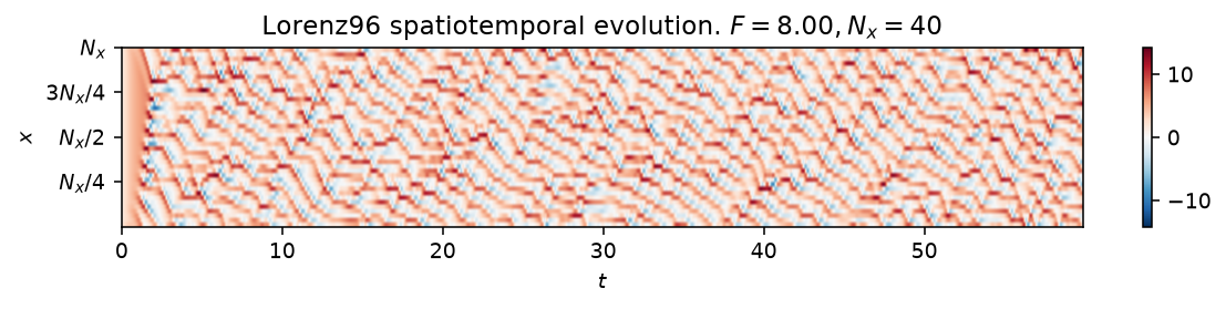
Lorenz96 spatiotemporal evolution

Space-time diagram of the 40-variable lattice at \(F=8\), past the transient: colour encodes \(x_i(t)\), with red and blue the positive and negative extremes. The travelling, roughly periodic wave packets are the model's analogue of synoptic-scale weather systems.

Quickstart

from dynamodels.physical import Lorenz96

model = Lorenz96(Nx=40, F=8., dt=0.01)
psi, t = model.time_integrate(Nt=6000)
model.update_history(psi, t)
model.visualize_spatiotemporal_hist()
model.close()

Three components are observable by default (observed_idx=[0, Nx//2, Nx-1]); pass observed_idx to choose others.

Nonlinear diagnostics

ntsa characterization of Lorenz96

Diagnostics from ntsa.characterize on a single lattice site, left to right: the observable time series with a zoomed inset; power spectral density; the 3-D delay-embedded portrait; the first-return map of the maxima; a plane-crossing Poincare section; a recurrence plot; a 3-D classical-MDS embedding of the full 40-variable state; and the Lyapunov spectrum (analytic Jacobian, since time_derivative is available).

Reference

Lorenz, E. N. (1996). Predictability: a problem partly solved. Proceedings of the Seminar on Predictability, Vol. 1, ECMWF, Reading, UK, 1-18.

API

dynamodels.physical.lorenz96.Lorenz96

Bases: Model

Lorenz (1996) system — chaotic model of \(N_x\) variables on a periodic lattice.

\[ \dot{x}_i = \left(x_{i+1} - x_{i-2}\right) x_{i-1} - x_i + F, \qquad i = 0, \dots, N_x - 1, \]

with indices taken cyclically modulo \(N_x\) (i.e. \(x_{-1} = x_{N_x - 1}\), \(x_{-2} = x_{N_x - 2}\) and \(x_{N_x} = x_0\)). Each variable is coupled quadratically to its two upstream neighbours, damped linearly (\(-x_i\)) and driven by a constant forcing \(F\). With the classical parameters (\(N_x = 40\), \(F = 8\)) the system is chaotic.

References

Lorenz (1996). Predictability: a problem partly solved. Proc. Seminar on Predictability, Vol. 1, ECMWF, Reading, UK, 1-18.

Source code in dynamodels/physical/lorenz96.py
 25
 26
 27
 28
 29
 30
 31
 32
 33
 34
 35
 36
 37
 38
 39
 40
 41
 42
 43
 44
 45
 46
 47
 48
 49
 50
 51
 52
 53
 54
 55
 56
 57
 58
 59
 60
 61
 62
 63
 64
 65
 66
 67
 68
 69
 70
 71
 72
 73
 74
 75
 76
 77
 78
 79
 80
 81
 82
 83
 84
 85
 86
 87
 88
 89
 90
 91
 92
 93
 94
 95
 96
 97
 98
 99
100
101
102
103
104
105
106
107
108
109
110
111
112
113
114
115
116
117
118
119
120
121
122
123
124
125
126
127
128
129
130
131
132
133
134
135
136
137
138
139
140
141
142
143
144
145
146
147
148
149
150
151
152
153
154
155
156
157
158
159
160
161
162
163
164
165
166
167
168
169
170
171
172
173
174
175
176
177
178
179
180
181
182
183
184
185
186
187
188
class Lorenz96(Model):
    r"""Lorenz (1996) system — chaotic model of $N_x$ variables on a periodic lattice.

    $$
    \dot{x}_i = \left(x_{i+1} - x_{i-2}\right) x_{i-1} - x_i + F,
    \qquad i = 0, \dots, N_x - 1,
    $$

    with indices taken cyclically modulo $N_x$ (i.e. $x_{-1} = x_{N_x - 1}$,
    $x_{-2} = x_{N_x - 2}$ and $x_{N_x} = x_0$). Each variable is coupled
    quadratically to its two upstream neighbours, damped linearly ($-x_i$) and
    driven by a constant forcing $F$. With the classical parameters
    ($N_x = 40$, $F = 8$) the system is chaotic.

    References
    ----------
    Lorenz (1996). Predictability: a problem partly solved. *Proc. Seminar on
    Predictability*, Vol. 1, ECMWF, Reading, UK, 1-18.
    """

    # --- Core Physics Parameters ---
    t_lyap = 1.67 ** (-1)
    t_transient = 40 * t_lyap
    t_CR = 4 * t_lyap
    Nq = 3

    F = 8.0
    Nx = 40

    # --- Ensemble/Augmentation Configuration Placeholders (Required by Model Base Class) ---
    # These are populated later, but required for property calculations in Model
    est_a: list[str] = []

    # --- Parameter and State Labels ---
    extra_print_params = ['observed_idx', 'Nq', 't_lyap', 'Nx']
    fixed_params = ['Nx']
    params = ['F']

    # __________________________ Init method ___________________________ #
    def __init__(self, **model_dict):

        self.Nx = model_dict.pop('Nx', 40)
        psi0 = model_dict.pop('psi0', np.array([1.6] + [1.0] * (self.Nx - 1)))
        dt = model_dict.pop('dt', 0.01)

        self.observed_idx = model_dict.pop('observed_idx', [0, self.Nx//2, self.Nx-1]) # Default to observing three dimensions if not specified
        self.Nq = len(self.observed_idx)

        super().__init__(psi0=psi0, dt=dt, integrator_class=IVPIntegrator, **model_dict)

        # measured 1/lambda1 at this F (Nx=10 table only; set once — params change
        # by re-instantiation)
        if self.Nx == 10:
            self.t_lyap = self.t_lyap_from_table(self.F, _LAM1_MEASURED_NX10, Lorenz96.t_lyap)

        self.alpha_labels = dict(F='$F$')


    # _______________ Lorenz63 specific properties and methods ________________ #

    @property
    def state_labels(self):
        return [f'$x_{{{kk}}}$' for kk in range(self.Nx)]


    @property
    def obs_labels(self):
        return [self.state_labels[kk] for kk in self.observed_idx]

    def get_observables(self, Nt=1, **kwargs):
        if Nt == 1:
            return self.hist[-1, self.observed_idx, :]
        else:
            return self.hist[-Nt:, self.observed_idx, :]


    @staticmethod
    def time_derivative(t, psi, Nx, F):
        """
        Calculates the time derivative of the Lorenz 96 system (see class docstring).
        """

        x = psi[:Nx]

        dx = (np.roll(x, -1) - np.roll(x, 2)) * np.roll(x, 1) - x + F

        if len(psi) > Nx:
             dx = np.concatenate((dx, np.zeros(len(psi) - Nx)))

        return dx


    def visualize_spatiotemporal_hist(self, y_hist=None, t=None, nrows=None, averaged=False,
                                      reference_y=1.0, reference_t: float = 1.0, **kwargs):

        if y_hist is None:
            y_hist = self.hist[:, :self.Nx]

        if t is None:
            t = self.hist_t

        (t,), t_lbl = normalized_time(reference_t, t)
        assert t is not None
        if reference_y != 1.0:
            y_hist = y_hist / reference_y

        if not averaged:
            if nrows is None:
                nrows = min(10, y_hist.shape[-1])

            fig = plt.figure(figsize=(10, 1.5 * nrows))
            axs = fig.subplots(nrows=nrows, sharey=True, sharex=True)
            if nrows == 1:
                axs = [axs]

            lim = np.max(abs(y_hist))

            for mi, ax in enumerate(axs):
                im = ax.imshow(y_hist[:, :, mi].T,
                            aspect='auto', origin='lower',
                            cmap='RdBu_r', vmin=-lim, vmax=lim,
                            extent=[t[0], t[-1], 0, self.Nx])  # TRANSPOSE


            axs[0].set(title=rf"Lorenz96 spatiotemporal evolution. $F={self.F:.2f}, N_x={self.Nx}$")
            axs[-1].set(xlabel=t_lbl)

            fig.colorbar(im, ax=axs, orientation='vertical', shrink=1/nrows) #type: ignore
        else:
            # Averaged ensemble visualization
            y_mean_hist = np.mean(y_hist, axis=-1)

            fig, axs = plt.subplots(nrows=2, figsize=(10, 6), sharex=True)

            # Mean evolution
            lim_mean = np.max(abs(y_mean_hist))
            im0 = axs[0].imshow(y_mean_hist.T,
                                aspect='auto', origin='lower',
                                cmap='RdBu_r', vmin=-lim_mean, vmax=lim_mean,
                                extent=[t[0], t[-1], 0, self.Nx])  # TRANSPOSE
            axs[0].set(title=rf"Lorenz96 averaged spatiotemporal evolution (mean and std). $F={self.F:.2f}, N_x={self.Nx}$")
            fig.colorbar(im0, ax=axs[0], orientation='vertical')

            # Deviation covariance evolution

            var_ensemble = np.var(y_hist, axis=-1, ddof=1).T            # (Nt, Nx)
            var_ensemble = np.sqrt(var_ensemble)                     # Standard deviation

            lim_dev = np.max(abs(var_ensemble))
            im1 = axs[1].imshow(var_ensemble,  # Plot covariance of deviations
                                aspect='auto', origin='lower',
                                cmap='magma', vmin=0, vmax=lim_dev,
                                extent=[t[0], t[-1], 0, self.Nx])  # TRANSPOSE

            fig.colorbar(im1, ax=axs[1], orientation='vertical')
        # add the ticks and labels

        # Set spatial ticks as multiples of L
        ticks = (np.arange(4) + 1)* self.Nx/4
        tick_labels = [r"$N_x/4$", r"$N_x/2$", r"$3N_x/4$",r"$N_x$"]
        for ax in axs:
            ax.set(ylabel="$x$", yticks=ticks, yticklabels=tick_labels)

time_derivative(t, psi, Nx, F) staticmethod

Calculates the time derivative of the Lorenz 96 system (see class docstring).

Source code in dynamodels/physical/lorenz96.py
101
102
103
104
105
106
107
108
109
110
111
112
113
114
@staticmethod
def time_derivative(t, psi, Nx, F):
    """
    Calculates the time derivative of the Lorenz 96 system (see class docstring).
    """

    x = psi[:Nx]

    dx = (np.roll(x, -1) - np.roll(x, 2)) * np.roll(x, 1) - x + F

    if len(psi) > Nx:
         dx = np.concatenate((dx, np.zeros(len(psi) - Nx)))

    return dx