Rijke tube

The Rijke tube is a longitudinal thermoacoustic system: a heated gauze inside a tube couples an unsteady heat release to the acoustic field, and the two can lock into a self-sustained oscillation. The acoustic velocity and pressure are expanded on \(N_m\) Galerkin modes, giving modal ODEs for each mode's amplitude \(\eta_j\) and its rate \(\mu_j\), damped at rate \(\zeta_j = C_1 j^2 + C_2 \sqrt{j}\) and driven by the heat release projected onto the modes. The heat release itself follows a gain-delay law: it depends on the acoustic velocity at the flame location \(x_f\), delayed by a time \(\tau\) and related through a square-root (\(\text{law}='sqrt'\)) or a saturating arctangent (\(\text{law}='tan'\)) nonlinearity. The delay is realized numerically by advecting the velocity along an auxiliary field discretized with \(N_c\) Chebyshev collocation points. The estimable parameters are the heat-release intensity \(\beta\), the delay \(\tau\), the damping coefficients \(C_1\), \(C_2\), and the saturation \(\kappa\); the observables are the pressure at Nq microphone locations. The full modal equations are in the API reference below.

\(\beta\) alone routes the system through a sequence of regimes, four of which are pre-tabulated in CASES and selected with case='...'.

Quickstart

from dynamodels.physical import Rijke

model = Rijke(case='limit_cycle', dt=1e-4)
psi, t = model.time_integrate(Nt=5000)
model.update_history(psi, t)
model.visualize_observable_hist()
model.close()

Regimes

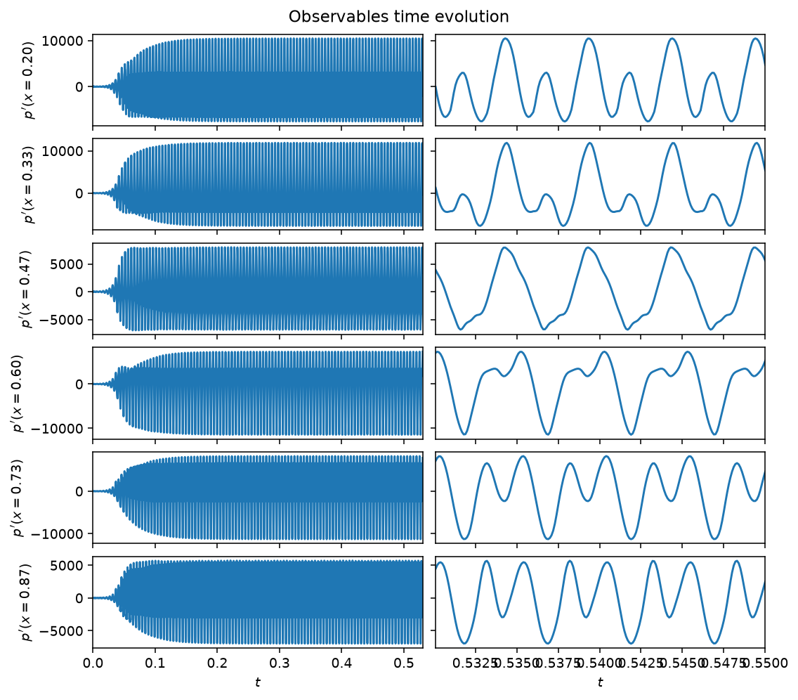
case='limit_cycle' (\(\beta=4\), the class default): a period-2 limit cycle, its two harmonics visible as the alternating tall/short peaks in the zoomed panel.

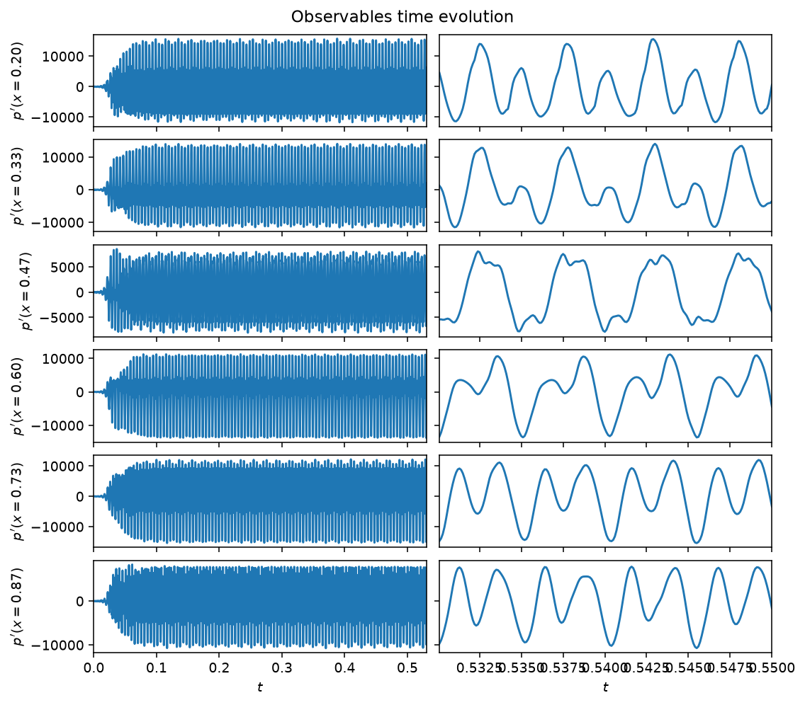
case='frequency_locked' (\(\beta=8\)): two modes lock onto a common period, giving the slow amplitude-modulated (beating) waveform in the zoomed panel.

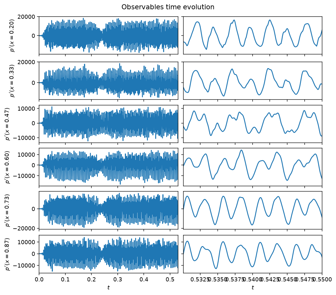
case='chaotic' (\(\beta=12\), measured \(\lambda_1=161\,\mathrm{s^{-1}}\)): an aperiodic, broadband pressure signal.

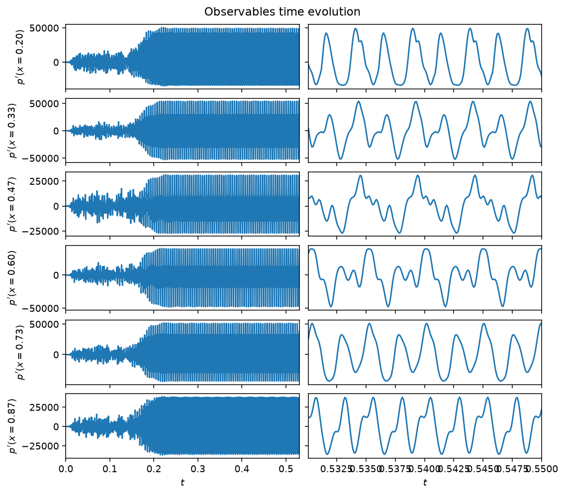
case='relaminarized' (\(\beta=18\)): past the chaotic window, the system relaminarizes onto a period-3 limit cycle at a larger amplitude.

The microphone traces above are samples of a field that fills the whole tube. For the chaotic case, an animation shows both at once:

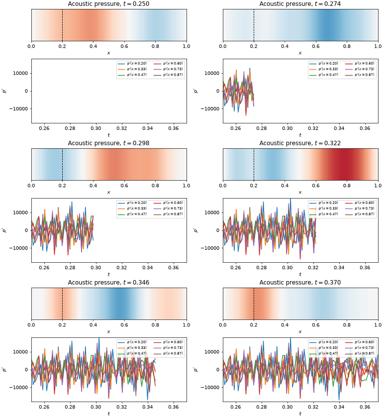
case='chaotic' (\(\beta=12\)), past the transient. Top: the acoustic pressure \(p'(x,t)\) along the tube, with the flame location \(x_f=0.2\) dashed. Bottom: the same field sampled at the six microphones. The pressure node imposed by the open ends stays fixed while the amplitude varies aperiodically. The Rijke tube tutorial builds this figure step by step.

Nonlinear diagnostics

Diagnostics from ntsa.characterize on the limit-cycle case, left to right: the observable time series with a zoomed inset; power spectral density; the 3-D delay-embedded portrait; the first-return map of the maxima; a plane-crossing Poincare section; a recurrence plot; and a 3-D classical-MDS embedding of the full modal state. The last panel (leading Lyapunov exponent) is blank here: for a limit cycle this close to neutral, the perturbation-growth fit's own reliability guard abstains rather than report a noisy estimate -- see Analysing a model.

Reference

Novoa, A., & Magri, L. (2022). Real-time thermoacoustic data assimilation. Journal of Fluid Mechanics, 948, A35. doi:10.1017/jfm.2022.653

API

dynamodels.physical.rijke.Rijke

Bases: Model

Rijke tube — longitudinal thermoacoustic low-order model.

The acoustic velocity and pressure perturbations are expanded on \(N_m\) Galerkin modes with wavenumbers \(k_j = j\pi/L\),

\[ u'(x, t) = \sum_{j=1}^{N_m} \eta_j(t) \cos(k_j x), \qquad p'(x, t) = -\sum_{j=1}^{N_m} \mu_j(t) \sin(k_j x), \]

giving the modal ODEs

\[ \dot{\eta}_j = \frac{k_j}{\bar\rho}\, \mu_j, \qquad \dot{\mu}_j = -k_j\, \bar\rho\, \bar{c}^2\, \eta_j - \frac{\bar{c}}{L}\, \zeta_j\, \mu_j + \dot{q}_j, \qquad \zeta_j = C_1\, j^2 + C_2\, \sqrt{j}, \]

where \(\bar\rho\), \(\bar{c}\) (and \(\bar{u}\), \(\bar{p}\), \(\bar\gamma\) below) are fixed mean-flow properties, weight-averaged across the temperature jump at the flame location \(x_f\), and \(\zeta_j\) is the modal damping. The heat release is projected onto the modes as

\[ \dot{q}_j = -\frac{2 (\bar\gamma - 1)}{L} \sin(k_j x_f)\, \dot{q}'(x_f, t), \]

with a gain–delay law relating \(\dot{q}'\) to the (time-delayed) acoustic velocity at the flame, \(u_f(t) \equiv u'(x_f, t - \tau)\): a square-root law (law='sqrt')

\[ \dot{q}'(x_f, t) = \bar{p}\, \bar{u}\, \beta \left[ \sqrt{\left| \tfrac{1}{3} + u_f(t) / \bar{u} \right|} - \sqrt{\tfrac{1}{3}} \right], \]

or a saturating arctangent law (law='tan')

\[ \dot{q}'(x_f, t) = \beta \sqrt{\beta / \kappa}\, \arctan\!\left( \sqrt{\beta / \kappa}\, u_f(t) \right). \]

The delay \(\tau\) is realized by advecting \(u'(x_f, t)\) along an auxiliary field discretized with \(N_c\) Chebyshev collocation points, and interpolating it at the point corresponding to the elapsed delay to obtain \(u_f(t)\).

The estimable parameters are \(\beta\), \(\tau\), the damping coefficients \(C_1\), \(C_2\), and \(\kappa\) (only active for law='tan'). The observables are the pressure at Nq microphone locations.

Four named regimes along the \(\beta\) route are pre-tabulated in CASES and selected with case='...': 'limit_cycle' (the class default, a period-2 limit cycle), 'frequency_locked', 'chaotic', and 'relaminarized' (a period-3 limit cycle). Explicit keyword arguments override a case's values.

References

Nóvoa & Magri (2022). Real-time thermoacoustic data assimilation. J. Fluid Mech., 948, A35. DOI: 10.1017/jfm.2022.653.

Source code in dynamodels/physical/rijke.py

class Rijke(Model):
    r"""Rijke tube — longitudinal thermoacoustic low-order model.

    The acoustic velocity and pressure perturbations are expanded on $N_m$
    Galerkin modes with wavenumbers $k_j = j\pi/L$,

    $$
    u'(x, t) = \sum_{j=1}^{N_m} \eta_j(t) \cos(k_j x), \qquad
    p'(x, t) = -\sum_{j=1}^{N_m} \mu_j(t) \sin(k_j x),
    $$

    giving the modal ODEs

    $$
    \dot{\eta}_j = \frac{k_j}{\bar\rho}\, \mu_j, \qquad
    \dot{\mu}_j = -k_j\, \bar\rho\, \bar{c}^2\, \eta_j
    - \frac{\bar{c}}{L}\, \zeta_j\, \mu_j + \dot{q}_j,
    \qquad \zeta_j = C_1\, j^2 + C_2\, \sqrt{j},
    $$

    where $\bar\rho$, $\bar{c}$ (and $\bar{u}$, $\bar{p}$, $\bar\gamma$ below) are
    fixed mean-flow properties, weight-averaged across the temperature jump at the
    flame location $x_f$, and $\zeta_j$ is the modal damping. The heat release is
    projected onto the modes as

    $$
    \dot{q}_j = -\frac{2 (\bar\gamma - 1)}{L} \sin(k_j x_f)\, \dot{q}'(x_f, t),
    $$

    with a gain–delay law relating $\dot{q}'$ to the (time-delayed) acoustic
    velocity at the flame, $u_f(t) \equiv u'(x_f, t - \tau)$: a square-root law
    (``law='sqrt'``)

    $$
    \dot{q}'(x_f, t) = \bar{p}\, \bar{u}\, \beta \left[
    \sqrt{\left| \tfrac{1}{3} + u_f(t) / \bar{u} \right|} - \sqrt{\tfrac{1}{3}}
    \right],
    $$

    or a saturating arctangent law (``law='tan'``)

    $$
    \dot{q}'(x_f, t) = \beta \sqrt{\beta / \kappa}\,
    \arctan\!\left( \sqrt{\beta / \kappa}\, u_f(t) \right).
    $$

    The delay $\tau$ is realized by advecting $u'(x_f, t)$ along an auxiliary
    field discretized with $N_c$ Chebyshev collocation points, and interpolating
    it at the point corresponding to the elapsed delay to obtain $u_f(t)$.

    The estimable parameters are $\beta$, $\tau$, the damping coefficients $C_1$,
    $C_2$, and $\kappa$ (only active for ``law='tan'``). The observables are the
    pressure at ``Nq`` microphone locations.

    Four named regimes along the $\beta$ route are pre-tabulated in `CASES` and
    selected with ``case='...'``: ``'limit_cycle'`` (the class default, a period-2
    limit cycle), ``'frequency_locked'``, ``'chaotic'``, and ``'relaminarized'``
    (a period-3 limit cycle). Explicit keyword arguments override a case's values.

    References
    ----------
    Nóvoa & Magri (2022). Real-time thermoacoustic data assimilation.
    *J. Fluid Mech.*, 948, A35. [DOI: 10.1017/jfm.2022.653](https://doi.org/10.1017/jfm.2022.653).
    """

    # name: str = 'Rijke'
    t_transient = .25
    t_CR = 0.02
    t_lyap = t_CR  # overwritten per instance with measured 1/lambda1(beta) when chaotic

    Nm = 10
    Nc = 10
    Nq = 6

    beta, tau = 4.0, 1.5E-3
    C1, C2 = 0.05, 0.01
    kappa = 1E5
    xf, L = 0.2, 1.
    law = 'sqrt'

    # --- Parameter and fixed parameter lists ---
    params = ['beta', 'tau', 'C1', 'C2', 'kappa']
    fixed_params = ['cosomjxf', 'Dc', 'gc', 'jpiL', 'L',
                    'law', 'meanFlow', 'Nc', 'Nm', 'tau_adv', 'sinomjxf']

    extra_print_params = ['law', 'Nm', 'Nc', 'xf', 'L']

    def __init__(self, **model_dict):

        case = model_dict.pop('case', None)
        if case is not None:
            if case not in CASES:
                raise ValueError(f"Unknown case '{case}'. Must be one of {list(CASES)}.")
            for key, val in CASES[case].items():
                model_dict.setdefault(key, val)  # explicit kwargs win over the case

        if 'psi0' not in model_dict.keys():
            if 'Nm' in model_dict.keys():
                Nm = model_dict['Nm']
            else:
                Nm = self.Nm
            if 'Nc' in model_dict.keys():
                Nc = model_dict['Nc']
            else:
                Nc = self.Nc
            model_dict['psi0'] = .05 * np.hstack([np.ones(2 * Nm), np.zeros(Nc)])

        dt = model_dict.pop('dt', 1E-4)

        self.tau_adv = self.tau


        self.alpha_labels = dict(beta='$\\beta$', tau='$\\tau$', C1='$C_1$', C2='$C_2$', kappa='$\\kappa$')
        self.alpha_lims =  dict(beta=(0.01, 5), tau=(1E-6, self.tau_adv), C1=(0., 1.), C2=(0., 1.), kappa=(1E3, 1E8))


        # Chebyshev modes
        self.Dc, self.gc = Cheb(self.Nc, getg=True)

        # Microphone locations
        self.x_mic = np.linspace(self.xf, self.L, self.Nq + 1)[:-1]

        # Define modes frequency of each mode and sin cos etc
        jj = np.arange(1, self.Nm + 1)
        self.jpiL = jj * np.pi / self.L
        self.sinomjxf = np.sin(self.jpiL * self.xf)
        self.cosomjxf = np.cos(self.jpiL * self.xf)

        # Mean Flow Properties
        def weight_avg(y1, y2):
            return self.xf / self.L * y1 + (1. - self.xf / self.L) * y2

        self.meanFlow = dict(u=weight_avg(10, 11.1643), p=101300.,
                             gamma=1.4, T=weight_avg(300, 446.5282), R=287.1)
        self.meanFlow['rho'] = self.meanFlow['p'] / (self.meanFlow['R'] * self.meanFlow['T'])
        self.meanFlow['c'] = np.sqrt(self.meanFlow['gamma'] * self.meanFlow['R'] * self.meanFlow['T'])

        super().__init__(dt=dt, integrator_class=IVPIntegrator, **model_dict)

        # measured 1/lambda1 at this beta (set once: params change by re-instantiation)
        self.t_lyap = self.t_lyap_from_table(self.beta, _LAM1_MEASURED, Rijke.t_lyap)

        # Wave input_parameters ############################################################################################
        # c1: 347.2492    p1: 1.0131e+05      rho1: 1.1762    u1: 10          M1: 0.0288          T1: 300
        # c2: 423.6479    p2: 101300          rho2: 0.7902    u2: 11.1643     M2: 0.0264          T2: 446.5282
        # Tau: 0.0320     Td: 0.0038          Tu: 0.0012      R_in: -0.9970   R_out: -0.9970      Su: 0.9000
        # Q_bar: 5000     R_gas: 287.1000     gamma: 1.4000
        ##############################################################################################################

    def modify_settings(self):
        if 'tau' in self.est_alpha:
            extra_Nc = 50 - self.Nc
            self.tau_adv, self.Nc = 1E-2, 50
            self.alpha_lims = dict(tau=(1E-6, self.tau_adv)) # this updates the limits for tau to reflect the new tau_adv value

            psi = self.current_state

            new_psi = np.concatenate([psi,
                                      np.zeros((extra_Nc, psi.shape[-1]))], axis=0)

            self.psi0 = np.mean(new_psi, axis=1, keepdims=True)

            self.Dc, self.gc = Cheb(self.Nc, getg=True)

            self.update_history(t=0., psi=self.psi0, reset=True)

            self.set_fixed_params()

    # _______________ Rijke specific properties and methods ________________ #
    @property
    def obs_labels(self, loc=None):
        if loc is None:
            loc = np.expand_dims(self.x_mic, axis=1)
        return [f"$p'(x = {x:.2f})$" for x in loc[:, 0]]

    @property
    def state_labels(self):
        lbls0 = [f"$\\eta_{j}$" for j in np.arange(self.Nm)]
        lbls1 = ["$\\dot{\\eta}$" + f"$_{j}$" for j in np.arange(self.Nm)]
        lbls2 = [f"$\\nu_{j}$" for j in np.arange(self.Nc)]
        return lbls0 + lbls1 + lbls2

    def get_observables(self, Nt=1, loc=None, **kwargs):
        if loc is None:
            loc = self.x_mic
        elif isinstance(loc, str) and loc == "all":
            loc = np.linspace(0, self.L, 100)[:-1]

        loc = np.expand_dims(loc, axis=1)
        om = np.array([self.jpiL])
        mu = self.hist[-Nt:, self.Nm:2 * self.Nm, :]

        # Compute acoustic pressure and velocity at locations
        p_mic = -np.dot(np.sin(np.dot(loc, om)), mu)
        p_mic = p_mic.transpose(1, 0, 2)
        if Nt == 1:
            p_mic = p_mic[0]
        return p_mic

    @staticmethod
    def time_derivative(t, psi,
                        C1, C2, beta, kappa, tau,
                        cosomjxf, Dc, gc, jpiL, L, law, meanFlow, Nc, Nm, tau_adv, sinomjxf):
        r"""Time derivative of the Rijke tube governing equations (see class docstring).

        Parameters
        ----------
        t : float
            Current time.
        psi : ndarray
            Augmented state vector; the first ``2 * Nm + Nc`` entries are
            ``[eta (Nm,), mu (Nm,), v (Nc,)]``.
        C1, C2 : float
            Modal damping coefficients, $\zeta_j = C_1 j^2 + C_2 \sqrt{j}$.
        beta : float
            Heat-release intensity.
        kappa : float
            Saturation parameter used by the ``'tan'`` heat-release law.
        tau : float
            Time delay of the flame response.
        cosomjxf, sinomjxf : ndarray
            Precomputed $\cos(k_j x_f)$, $\sin(k_j x_f)$ for each mode $j$, used
            respectively to evaluate $u'(x_f, t)$ and to project the heat release
            onto the $\mu$ modes.
        Dc, gc : ndarray
            Chebyshev differentiation matrix and collocation points used to
            advect the delay line.
        jpiL : ndarray
            Modal wavenumbers $k_j = j\pi/L$.
        L : float
            Tube length.
        law : str
            Heat-release law, ``'sqrt'`` or ``'tan'``.
        meanFlow : dict
            Mean-flow properties at the flame ($\bar\rho$, $\bar u$, $\bar p$,
            $\bar c$, $\bar\gamma$, $\bar T$).
        Nc : int
            Number of Chebyshev modes discretizing the delay line.
        Nm : int
            Number of Galerkin modes.
        tau_adv : float
            Reference advection time spanned by the delay line.

        Returns
        -------
        ndarray
            Concatenated time derivative of the augmented state vector.
        """
        eta, mu, v = psi[:Nm], psi[Nm: 2 * Nm], psi[2 * Nm: 2 * Nm + Nc]

        # Advection equation boundary conditions
        v2 = np.hstack((np.dot(eta, cosomjxf), v))

        # Evaluate u(t_interp-tau) i.e. velocity at the flame at t_interp - tau
        x_tau = tau / tau_adv
        if x_tau < 1:
            f = splrep(gc, v2)
            u_tau = splev(x_tau, f)
        elif x_tau == 1:  # if no tau estimation, bypass interpolation to speed up code
            u_tau = v2[-1]
        else:
            raise Exception(f"tau = {tau} can't_interp be larger than tau_adv = {tau_adv}")

        # Compute damping and heat release law
        zeta = C1 * (jpiL * L / np.pi) ** 2 + C2 * (jpiL * L / np.pi) ** .5

        MF = meanFlow.copy()  # Physical properties
        if law == 'sqrt':
            q_dot = MF['p'] * MF['u'] * beta * (
                    np.sqrt(abs(1. / 3 + u_tau / MF['u'])) - np.sqrt(1. / 3))  # [W/m2]=[m/s3]
        elif law == 'tan':
            q_dot = beta * np.sqrt(beta / kappa) * np.arctan(np.sqrt(beta / kappa) * u_tau)  # [m / s3]
        else:
            raise ValueError(f'Law "{law}" not defined')
        q_dot *= -2. * (MF['gamma'] - 1.) / L * sinomjxf  # [Pa/s]

        # governing equations
        deta_dt = jpiL / MF['rho'] * mu
        dmu_dt = - jpiL * MF['gamma'] * MF['p'] * eta - MF['c'] / L * zeta * mu + q_dot
        dv_dt = - 2. / tau_adv * np.dot(Dc, v2)

        return np.concatenate((deta_dt, dmu_dt, dv_dt[1:], np.zeros(len(psi) - (2 * Nm + Nc))))



    def visualize_spatiotemporal_hist(self, y_hist=None, t=None, nrows=None, averaged=False,
                                      reference_y=1.0, reference_t: float = 1.0, **kwargs):
        """
        Visualize the spatiotemporal evolution of the Rijke tube model in the physical space.
        """

        if y_hist is None:
            Nt = int(self.t_CR // self.dt)
            y_hist = self.get_observable_hist(loc="all", Nt=Nt)

        if t is None:
            t = self.hist_t

        (t,), t_lbl = normalized_time(reference_t, t)
        assert t is not None
        if reference_y != 1.0:
            y_hist = y_hist / reference_y


        # Set spatial ticks as multiples of L
        ticks = np.arange(5)* self.L/4
        # tick_labels = [r"$L/4$", r"$L/2$", r"$3L/4$",r"$L$"]

        if not averaged:
            if nrows is None:
                nrows = min(10, y_hist.shape[-1])

            fig = plt.figure(figsize=(10, 1.5 * nrows))
            axs = fig.subplots(nrows=nrows, sharey=True, sharex=True)
            if nrows == 1:
                axs = [axs]

            lim = np.max(abs(y_hist))
            for mi, ax in enumerate(axs):
                im = ax.imshow(y_hist[:, :, mi].T,
                            aspect='auto', origin='lower',
                            cmap='RdBu_r',
                            vmin=-lim, vmax=lim,
                            extent=[t[0], t[-1], 0, self.L])
                ax.set(ylabel="$x$")
                ax.set_yticks(ticks)
                # ax.set_yticklabels(tick_labels)
            fig.colorbar(im, ax=axs, orientation='vertical', shrink=1/nrows) #type: ignore


            axs[0].set(title=rf"Rijke spatiotemporal evolution $x_f={self.xf}$")
            axs[-1].set(xlabel=t_lbl)

        else:
            # Averaged ensemble visualization
            y_mean_hist = np.mean(y_hist, axis=-1)

            fig, axs = plt.subplots(nrows=2, figsize=(10, 6), sharex=True)

            # Mean evolution
            lim_mean = np.max(abs(y_mean_hist))
            im0 = axs[0].imshow(y_mean_hist.T,
                                aspect='auto', origin='lower',
                                cmap='RdBu_r', vmin=-lim_mean, vmax=lim_mean,
                                extent=[t[0], t[-1], 0, self.L])

            axs[0].set(title=rf"Rijke spatiotemporal evolution (mean and std) $x_f={self.xf}$")
            fig.colorbar(im0, ax=axs[0], orientation='vertical')
            # Deviation covariance evolution in percentage

            var_ensemble = np.var(y_hist, axis=-1, ddof=1).T            # (Nt, Nx)
            var_ensemble = np.sqrt(var_ensemble)                     # Standard deviation
            lim_dev = np.max(var_ensemble)
            im1 = axs[1].imshow(var_ensemble,  # Plot covariance of deviations
                                aspect='auto', origin='lower',
                                cmap='magma', vmin=0, vmax=lim_dev,
                                extent=[t[0], t[-1], 0, self.L])

            axs[1].set(xlabel=t_lbl)
            fig.colorbar(im1, ax=axs[1], orientation='vertical')


            for ax in axs:
                ax.set(yticks=ticks, ylabel="$x$")

time_derivative(t, psi, C1, C2, beta, kappa, tau, cosomjxf, Dc, gc, jpiL, L, law, meanFlow, Nc, Nm, tau_adv, sinomjxf) staticmethod

Time derivative of the Rijke tube governing equations (see class docstring).

Parameters:

Name	Type	Description	Default
t	float	Current time.	required
psi	ndarray	Augmented state vector; the first 2 * Nm + Nc entries are [eta (Nm,), mu (Nm,), v (Nc,)].	required
C1	float	Modal damping coefficients, \(\zeta_j = C_1 j^2 + C_2 \sqrt{j}\).	required
C2	float	Modal damping coefficients, \(\zeta_j = C_1 j^2 + C_2 \sqrt{j}\).	required
beta	float	Heat-release intensity.	required
kappa	float	Saturation parameter used by the 'tan' heat-release law.	required
tau	float	Time delay of the flame response.	required
cosomjxf	ndarray	Precomputed \(\cos(k_j x_f)\), \(\sin(k_j x_f)\) for each mode \(j\), used respectively to evaluate \(u'(x_f, t)\) and to project the heat release onto the \(\mu\) modes.	required
sinomjxf	ndarray	Precomputed \(\cos(k_j x_f)\), \(\sin(k_j x_f)\) for each mode \(j\), used respectively to evaluate \(u'(x_f, t)\) and to project the heat release onto the \(\mu\) modes.	required
Dc	ndarray	Chebyshev differentiation matrix and collocation points used to advect the delay line.	required
gc	ndarray	Chebyshev differentiation matrix and collocation points used to advect the delay line.	required
jpiL	ndarray	Modal wavenumbers \(k_j = j\pi/L\).	required
L	float	Tube length.	required
law	str	Heat-release law, 'sqrt' or 'tan'.	required
meanFlow	dict	Mean-flow properties at the flame (\(\bar\rho\), \(\bar u\), \(\bar p\), \(\bar c\), \(\bar\gamma\), \(\bar T\)).	required
Nc	int	Number of Chebyshev modes discretizing the delay line.	required
Nm	int	Number of Galerkin modes.	required
tau_adv	float	Reference advection time spanned by the delay line.	required

Returns:

Type	Description
ndarray	Concatenated time derivative of the augmented state vector.

Source code in dynamodels/physical/rijke.py

@staticmethod
def time_derivative(t, psi,
                    C1, C2, beta, kappa, tau,
                    cosomjxf, Dc, gc, jpiL, L, law, meanFlow, Nc, Nm, tau_adv, sinomjxf):
    r"""Time derivative of the Rijke tube governing equations (see class docstring).

    Parameters
    ----------
    t : float
        Current time.
    psi : ndarray
        Augmented state vector; the first ``2 * Nm + Nc`` entries are
        ``[eta (Nm,), mu (Nm,), v (Nc,)]``.
    C1, C2 : float
        Modal damping coefficients, $\zeta_j = C_1 j^2 + C_2 \sqrt{j}$.
    beta : float
        Heat-release intensity.
    kappa : float
        Saturation parameter used by the ``'tan'`` heat-release law.
    tau : float
        Time delay of the flame response.
    cosomjxf, sinomjxf : ndarray
        Precomputed $\cos(k_j x_f)$, $\sin(k_j x_f)$ for each mode $j$, used
        respectively to evaluate $u'(x_f, t)$ and to project the heat release
        onto the $\mu$ modes.
    Dc, gc : ndarray
        Chebyshev differentiation matrix and collocation points used to
        advect the delay line.
    jpiL : ndarray
        Modal wavenumbers $k_j = j\pi/L$.
    L : float
        Tube length.
    law : str
        Heat-release law, ``'sqrt'`` or ``'tan'``.
    meanFlow : dict
        Mean-flow properties at the flame ($\bar\rho$, $\bar u$, $\bar p$,
        $\bar c$, $\bar\gamma$, $\bar T$).
    Nc : int
        Number of Chebyshev modes discretizing the delay line.
    Nm : int
        Number of Galerkin modes.
    tau_adv : float
        Reference advection time spanned by the delay line.

    Returns
    -------
    ndarray
        Concatenated time derivative of the augmented state vector.
    """
    eta, mu, v = psi[:Nm], psi[Nm: 2 * Nm], psi[2 * Nm: 2 * Nm + Nc]

    # Advection equation boundary conditions
    v2 = np.hstack((np.dot(eta, cosomjxf), v))

    # Evaluate u(t_interp-tau) i.e. velocity at the flame at t_interp - tau
    x_tau = tau / tau_adv
    if x_tau < 1:
        f = splrep(gc, v2)
        u_tau = splev(x_tau, f)
    elif x_tau == 1:  # if no tau estimation, bypass interpolation to speed up code
        u_tau = v2[-1]
    else:
        raise Exception(f"tau = {tau} can't_interp be larger than tau_adv = {tau_adv}")

    # Compute damping and heat release law
    zeta = C1 * (jpiL * L / np.pi) ** 2 + C2 * (jpiL * L / np.pi) ** .5

    MF = meanFlow.copy()  # Physical properties
    if law == 'sqrt':
        q_dot = MF['p'] * MF['u'] * beta * (
                np.sqrt(abs(1. / 3 + u_tau / MF['u'])) - np.sqrt(1. / 3))  # [W/m2]=[m/s3]
    elif law == 'tan':
        q_dot = beta * np.sqrt(beta / kappa) * np.arctan(np.sqrt(beta / kappa) * u_tau)  # [m / s3]
    else:
        raise ValueError(f'Law "{law}" not defined')
    q_dot *= -2. * (MF['gamma'] - 1.) / L * sinomjxf  # [Pa/s]

    # governing equations
    deta_dt = jpiL / MF['rho'] * mu
    dmu_dt = - jpiL * MF['gamma'] * MF['p'] * eta - MF['c'] / L * zeta * mu + q_dot
    dv_dt = - 2. / tau_adv * np.dot(Dc, v2)

    return np.concatenate((deta_dt, dmu_dt, dv_dt[1:], np.zeros(len(psi) - (2 * Nm + Nc))))

visualize_spatiotemporal_hist(y_hist=None, t=None, nrows=None, averaged=False, reference_y=1.0, reference_t=1.0, **kwargs)

Visualize the spatiotemporal evolution of the Rijke tube model in the physical space.

Source code in dynamodels/physical/rijke.py

def visualize_spatiotemporal_hist(self, y_hist=None, t=None, nrows=None, averaged=False,
                                  reference_y=1.0, reference_t: float = 1.0, **kwargs):
    """
    Visualize the spatiotemporal evolution of the Rijke tube model in the physical space.
    """

    if y_hist is None:
        Nt = int(self.t_CR // self.dt)
        y_hist = self.get_observable_hist(loc="all", Nt=Nt)

    if t is None:
        t = self.hist_t

    (t,), t_lbl = normalized_time(reference_t, t)
    assert t is not None
    if reference_y != 1.0:
        y_hist = y_hist / reference_y


    # Set spatial ticks as multiples of L
    ticks = np.arange(5)* self.L/4
    # tick_labels = [r"$L/4$", r"$L/2$", r"$3L/4$",r"$L$"]

    if not averaged:
        if nrows is None:
            nrows = min(10, y_hist.shape[-1])

        fig = plt.figure(figsize=(10, 1.5 * nrows))
        axs = fig.subplots(nrows=nrows, sharey=True, sharex=True)
        if nrows == 1:
            axs = [axs]

        lim = np.max(abs(y_hist))
        for mi, ax in enumerate(axs):
            im = ax.imshow(y_hist[:, :, mi].T,
                        aspect='auto', origin='lower',
                        cmap='RdBu_r',
                        vmin=-lim, vmax=lim,
                        extent=[t[0], t[-1], 0, self.L])
            ax.set(ylabel="$x$")
            ax.set_yticks(ticks)
            # ax.set_yticklabels(tick_labels)
        fig.colorbar(im, ax=axs, orientation='vertical', shrink=1/nrows) #type: ignore


        axs[0].set(title=rf"Rijke spatiotemporal evolution $x_f={self.xf}$")
        axs[-1].set(xlabel=t_lbl)

    else:
        # Averaged ensemble visualization
        y_mean_hist = np.mean(y_hist, axis=-1)

        fig, axs = plt.subplots(nrows=2, figsize=(10, 6), sharex=True)

        # Mean evolution
        lim_mean = np.max(abs(y_mean_hist))
        im0 = axs[0].imshow(y_mean_hist.T,
                            aspect='auto', origin='lower',
                            cmap='RdBu_r', vmin=-lim_mean, vmax=lim_mean,
                            extent=[t[0], t[-1], 0, self.L])

        axs[0].set(title=rf"Rijke spatiotemporal evolution (mean and std) $x_f={self.xf}$")
        fig.colorbar(im0, ax=axs[0], orientation='vertical')
        # Deviation covariance evolution in percentage

        var_ensemble = np.var(y_hist, axis=-1, ddof=1).T            # (Nt, Nx)
        var_ensemble = np.sqrt(var_ensemble)                     # Standard deviation
        lim_dev = np.max(var_ensemble)
        im1 = axs[1].imshow(var_ensemble,  # Plot covariance of deviations
                            aspect='auto', origin='lower',
                            cmap='magma', vmin=0, vmax=lim_dev,
                            extent=[t[0], t[-1], 0, self.L])

        axs[1].set(xlabel=t_lbl)
        fig.colorbar(im1, ax=axs[1], orientation='vertical')


        for ax in axs:
            ax.set(yticks=ticks, ylabel="$x$")