Model protocol
Every function takes a model by duck type — no base-class requirement.
dynamodels is the reference
implementation (and supplies the demo/test models), but any object with this
interface works:
| Requirement | Used for |
|---|---|
constructor Cls(psi0=..., dt=..., **params) |
respawn re-instantiation |
dt, t_transient, t_CR (optional t_lyap) |
run horizons and reference times |
Nphi, Nq, psi0 (Nphi, m), alpha0 dict, fixed_params, params |
state/parameter bookkeeping |
obs_labels, alpha_labels, name |
figure labels |
time_integrate(Nt) -> (psi, t), update_history(psi, t, reset=), hist, hist_t, get_observable_hist(), close() |
trajectory generation (run_long) |
time_derivative(t, psi, **params) + governing_eqns_params |
QR spectrum only (lyapunov_spectrum); discrete maps can still use leading_lyapunov |
The two baselines below implement the same system — Lorenz-63,
\(\dot{x} = \sigma (y - x)\), \(\dot{y} = x (\rho - z) - y\), \(\dot{z} = x y - \beta z\) —
by subclassing dynamodels.Model, which supplies all the history bookkeeping. The only
choice to make is who does the time stepping: hand scipy.solve_ivp a time_derivative
(continuous route), or step the state yourself in time_step (discrete route).
Baseline: continuous model (IVP)
Define the right-hand side; IVPIntegrator does the rest. Governing parameters must be
class attributes (the base constructor only absorbs kwargs whose names already exist on
the class), and time_derivative's argument names must match params exactly — the
integrator calls it as fun(t, psi, **params).
import numpy as np
from dynamodels import Model, IVPIntegrator


class Lorenz63IVP(Model):

    sigma = 10.
    rho = 28.
    beta = 8. / 3.
    params = ['sigma', 'rho', 'beta']

    t_lyap = 1 / 0.906
    t_transient = 10 * t_lyap
    t_CR = 4 * t_lyap
    Nq = 3
    obs_labels = ['$x$', '$y$', '$z$']
    alpha_labels = dict(sigma='$\\sigma$', rho='$\\rho$', beta='$\\beta$')

    def __init__(self, **model_dict):
        psi0 = model_dict.pop('psi0', np.array([1., 1., 1.]))
        dt = model_dict.pop('dt', 0.02)
        super().__init__(psi0=psi0, dt=dt, integrator_class=IVPIntegrator, **model_dict)

    @staticmethod
    def time_derivative(t, psi, sigma, rho, beta):
        x, y, z = psi[:3]
        dx = sigma * (y - x)
        dy = x * (rho - z) - y
        dz = x * y - beta * z
        return (dx, dy, dz) + (0,) * (len(psi) - 3)
The trailing zero padding keeps the derivative valid for augmented state vectors (parameter-estimation members appended after the physical state).
Baseline: discrete model (own time stepper)
Same system, but the model owns the stepping — here a fixed-step RK4 written out, standing
in for whatever scheme a map or spectral solver dictates (the shipped KS model steps with
ETDRK4 this way). DiscreteIntegrator calls time_step(Nt), which must return the state
history including the initial condition — shapes (Nt + 1, Nphi, m) and (Nt + 1,) —
starting from self.current_state; the integrator strips row 0.
from dynamodels import DiscreteIntegrator


class Lorenz63Map(Model):

    sigma = 10.
    rho = 28.
    beta = 8. / 3.
    params = ['sigma', 'rho', 'beta']

    t_lyap = 1 / 0.906
    t_transient = 10 * t_lyap
    t_CR = 4 * t_lyap
    Nq = 3
    obs_labels = ['$x$', '$y$', '$z$']
    alpha_labels = dict(sigma='$\\sigma$', rho='$\\rho$', beta='$\\beta$')

    def __init__(self, **model_dict):
        psi0 = model_dict.pop('psi0', np.array([1., 1., 1.]))
        dt = model_dict.pop('dt', 0.02)
        super().__init__(psi0=psi0, dt=dt, integrator_class=DiscreteIntegrator, **model_dict)

    def _rhs(self, psi):
        x, y, z = psi[:3]
        return np.stack([self.sigma * (y - x),
                         x * (self.rho - z) - y,
                         x * y - self.beta * z])

    def _rk4_step(self, psi):
        dt = self.dt
        k1 = self._rhs(psi)
        k2 = self._rhs(psi + dt / 2 * k1)
        k3 = self._rhs(psi + dt / 2 * k2)
        k4 = self._rhs(psi + dt * k3)
        return psi + dt / 6 * (k1 + 2 * k2 + 2 * k3 + k4)

    def time_step(self, Nt=10, averaged=False, alpha=None):
        psi = self.current_state
        if psi.ndim == 1:
            psi = psi[:, None]
        t = np.round(self.current_time + np.arange(Nt + 1) * self.dt, self.precision_t)
        out = [psi]
        for _ in range(Nt):
            out.append(self._rk4_step(out[-1]))
        return np.stack(out, axis=0), t  # (Nt + 1, Nphi, m): IC included
With no time_derivative, lyapunov_spectrum (the QR route) is unavailable —
leading_lyapunov still works, per the last table row.
Same surface either way
Every ntsa function sees the two routes identically:
from ntsa.characterize import characterize
from ntsa.tools import run_long

for model in (Lorenz63IVP(), Lorenz63Map()):
    t, y, psi = run_long(model, t_run=20 * model.t_lyap)
    print(type(model).__name__, y.shape)   # both: (1105, 3)
    model.close()

characterize([Lorenz63IVP(), Lorenz63Map()])   # one 8-panel diagnostic row per model
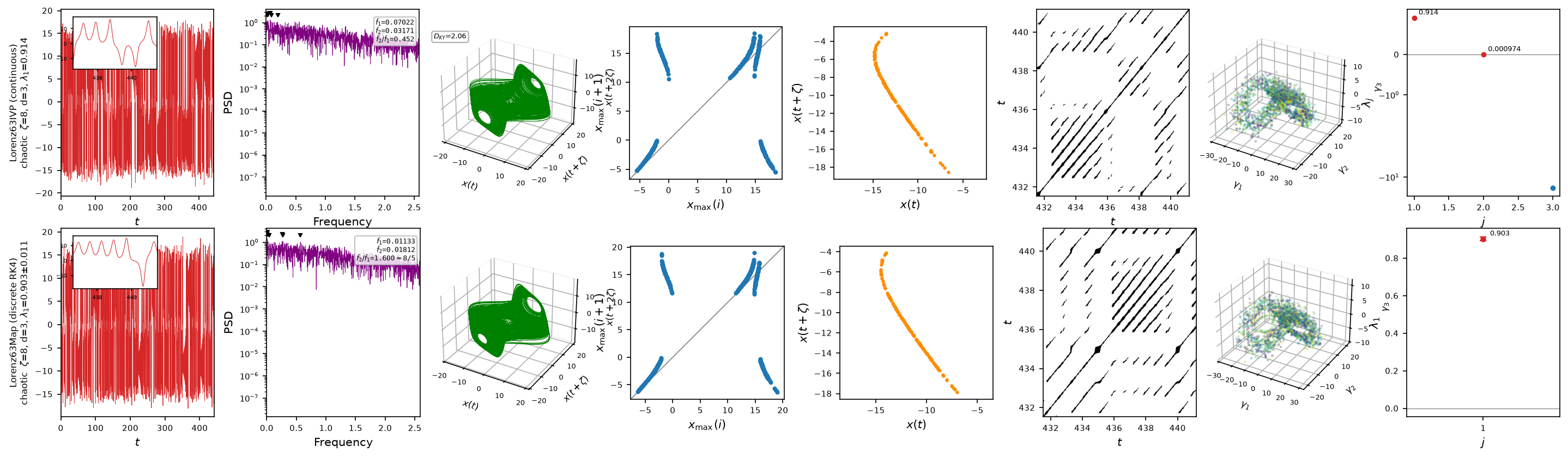
Same equations, two integration strategies: the delay portrait, return
map, PSD and recurrence plot line up almost exactly between the continuous
IVP baseline (top, \(\lambda_1=0.914\)) and the discrete RK4 baseline
(bottom, \(\lambda_1=0.903\)), both close to the reference \(0.906\). The last
panel differs because it must: Lorenz63IVP defines time_derivative, so
ntsa gets the full QR spectrum (three exponents); Lorenz63Map only
steps with time_step, so ntsa falls back to the single leading exponent
from leading_lyapunov — exactly the distinction in the protocol table's
last row.