Regime classification

A \(k\)-torus carries exactly \(k\) neutral exponents (\(|\lambda| <\) neutral_tol) and no positive one; chaos replaces one neutral direction with a positive exponent. Together with \(D_2\) on the attractor (\(\approx k\)) and on the section (\(\approx k-1\)) this fixes the torus dimension; the Lorenz96 Ruelle–Takens–Newhouse route is the worked example.

Decision tree

1. Fixed point — signal variance collapses (no sustained oscillation), or the full Lyapunov spectrum is entirely negative (decisive when integrator noise keeps the tail wiggling at a stable focus, e.g. Lorenz-63 at \(\rho\)=10: \(\lambda\) = [-0.6, -0.6, -12.5]).
2. Limit cycle, period-k — return-map local maxima form k \(\leq\) k_max distinct tight clusters. Checked before the Lyapunov step: k tight maxima levels over a long record are incompatible with chaos, whereas a perturbation-growth \(\lambda_1\) can read large and positive on a stable orbit through non-normal transient amplification (Rijke limit cycles read \(\lambda_1\) ~ 200 otherwise; leading_lyapunov additionally rejects fits whose saturation level sits far below the attractor diameter).
3. Chaotic — \(\lambda_1\) positive beyond the trust tolerance. characterize() classifies with the Benettin spectrum's \(\lambda_1\) whenever a spectrum was computed (it is convergence-controlled, std \(\approx\) 0), and with the perturbation-growth \(\lambda_1\) otherwise (whose member spread sets the 3\(\sigma\) part of the tolerance).
4. Otherwise: if a full spectrum is available, \(\geq\) 2 neutral exponents (\(|\lambda|\) < 2e-3) \(\to\) quasiperiodic (a 2-torus has two zero exponents; a locked periodic orbit exactly one — more robust than the PSD ratio test, whose limit_denominator(10) rationals are dense enough to "match" incommensurate ratios, e.g. L96 F=4.4: \(f_2/f_1\) = 0.552 \(\approx\) 5/9). Else dominant PSD frequencies rationally related \(\to\) frequency-locked; incommensurate \(\to\) quasiperiodic.

Caveat: the period-k count is the number of distinct maxima levels per cycle. A period-1 orbit whose waveform has several humps (e.g. the Rijke tube near its Hopf point: one large and one small maximum per acoustic period) is reported as period-k of the hump count. Disambiguate with the PSD in the panel text box: a genuine period-doubling shows a new subharmonic at f1/2; a multi-humped period-1 orbit shows only the harmonic comb of f1 (see the Rijke verification scripts in the romda repo, beta=0.4).

Bifurcation diagram: Lorenz-96 F-route

Local extrema of the observables against the swept parameter summarize the whole route the decision tree walks — bifurcation_sweep runs the sweep as one ensemble, plot_bifurcation draws it:

import numpy as np
from dynamodels.physical import Lorenz96
from ntsa.bifurcation import bifurcation_sweep, plot_bifurcation

model = Lorenz96(Nx=10)
values, peaks = bifurcation_sweep(model, 'F', np.linspace(0.5, 8., 120), extrema=('max', 'min'))
plot_bifurcation(values, peaks, model.alpha_labels['F'], model.obs_labels)

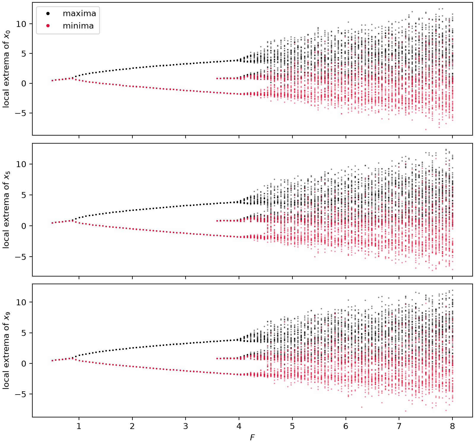
Read with the decision tree: maxima and minima coincide on the stable fixed point (\(F \lesssim 0.9\)); the Hopf bifurcation opens one tight level per branch (period-1 limit cycle); a second minima level appears near \(F \approx 3.6\) (a multi-humped waveform — the period-k caveat above); the levels smear into bands on the torus (\(F \approx 4.3\)) and fill out into broad scatter in chaos (\(F \gtrsim 4.6\)). The torus page walks this same route case by case. The three panels repeat the story at \(x_0\), \(x_5\), \(x_9\): the route is site-independent by the model's cyclic symmetry.

Measured \(\lambda_1\) tables in the model files

The dominant Lyapunov exponents measured here are stored in the dynamodels physical-model files (dynamodels/physical/{lorenz63,lorenz96,rijke}.py): a per-model _LAM1_MEASURED dict of chaotic parameter points, from which __init__ sets the instance's t_lyap = 1/$\lambda_1$ via Model.t_lyap_from_table (log-interpolated at the constructed sweep-parameter value). Class attributes keep the historical constants, so downstream users of the class constants (e.g. romda's scripts/mains) are unaffected; off-table configurations (limit cycles, tori, L96 with Nx != 10) keep them too. Values set once at construction — parameters change by re-instantiation. Extend the tables with {param: $\lambda_1$} pairs from converged runs; covered by test_t_lyap_tables in the dynamodels test suite.

Defaults

Quantity	Default
Delay \(\zeta\)	First local minimum of the average mutual information
Embedding dimension d	Kennel FNN with Rtol=10, Atol=2, threshold 1%
Recurrence threshold \(\varepsilon\)	10% of the max pairwise distance; the panel retargets to a fixed 10% recurrence rate (rr=0.10 quantile) when the density degenerates
Zoom inset / recurrence window	~5 / ~10 mean inter-maximum intervals (recurrence window clipped to [500, 2000] samples)
MDS / recurrence subsample	2000 points max
\(\lambda_1\) trust tolerance	\(\max(3\sigma,\ 10/T)\) (\(\lambda_1\) must exceed this to call chaos)
Spectrum integrator	RK4, dt = min(model.dt, 0.01)
Spectrum horizon	floor 200 * t_ref, extended (up to t_max = 20 * floor) until \(\lvert\lambda(T) - \lambda(T/2)\rvert < \max(\text{atol}, \text{rtol}\cdot\lvert\lambda\rvert)\) (atol = 2e-3, rtol = 5%) at two consecutive checks; warns if capped unconverged
Spectrum / leading-\(\lambda_1\) warmup	_settled_state: transient doubled (up to \(4\times\)) while stationary_start still sees amplitude drift in a 20*t_ref probe
Run horizon (characterize)	100 * model.t_CR, after discarding model.t_transient; residual drift trimmed by stationary_start

Notes

• The spectrum's neutral (along-flow) exponent converges to 0 only as O(1/T), so lyapunov_spectrum extends its horizon until the halving test passes: on a limit cycle the reported \(\lambda_1\) lands within ~atol–2atol of zero (VdP: +0.005 at the auto-chosen T\(\approx\)31 with the default atol=2e-3; +8e-4 with atol=5e-4, which runs to the t_max cap). Tighten atol (and raise t_max) for a cleaner zero; classification is unaffected (the \(\lambda_1\) trust floor \(\max(3\sigma,\ 10/T)\) sits far above it).
• The same O(1/T) bias is why a still-settling initial condition used to inflate \(\lambda_1\) on limit cycles: both lyapunov_spectrum and leading_lyapunov now warm up with _settled_state, which doubles the discarded transient until a probe run shows no amplitude drift (critical near Hopf points, where the decay rate vanishes and no fixed transient multiple is safe).
• covariant_lyapunov_vectors is a Ginelli (2007) TODO stub.
• lyapunov_spectrum needs time_derivative (continuous models); leading_lyapunov works for any Model (including discrete maps such as ESN or KS).
• characterize(..., spectrum=False) still estimates the dominant exponent automatically: the independent lyapunov switch (default 'auto') runs leading_lyapunov, which is based on perturbation growth alone — no Jacobian or tangent operator required. spectrum only controls the full Benettin QR pass; the spectrum's \(\lambda_1\) is used by the classification only as a fallback when the growth fit is rejected.
• Tutorial notebook: tutorial_ntsa.ipynb (full walkthrough on Lorenz63 + Lorenz96, executed).
• All randomness is seeded (np.random.default_rng(seed)).

References are collected on the theory overview.