Lyapunov exponents

Three routes, by what is available: the full spectrum needs the model's right-hand side (and ideally its Jacobian); the perturbation-growth estimate only needs a model that can be re-integrated; the Rosenstein estimate needs nothing but the measured series. The Kaplan–Yorke dimension follows from the spectrum.

Full spectrum: Benettin QR

The full spectrum comes from evolving the state jointly with a tangent basis \(\Psi \in \mathbb{R}^{N_\phi \times n_\mathrm{exp}}\) under the variational equation

\[ \dot{\psi} = f(\psi), \qquad \dot{\Psi} = J(\psi)\,\Psi, \qquad J = \frac{\partial f}{\partial \psi}, \]

(RK4, analytic \(J\) for Lorenz63/96, finite differences otherwise), with QR re-orthonormalization \(\Psi = QR\) every \(N_\mathrm{gs}\) steps. The exponents are the time-averaged log growth of the diagonal of \(R\) [Benettin et al. 1980]:

\[ \lambda_j = \lim_{T \to \infty} \frac{1}{T} \sum_{m} \ln R_{jj}^{(m)} . \]

Convergence control. The neutral (along-flow) exponent decays to zero only as \(\mathcal{O}(1/T)\), so the horizon is extended (up to t_max) until the halving test

\[ \left| \lambda_j(T) - \lambda_j(T/2) \right| < \max\!\left( \text{atol},\ \text{rtol} \cdot |\lambda_j| \right) \]

passes at two consecutive checks (one can be a phase coincidence).

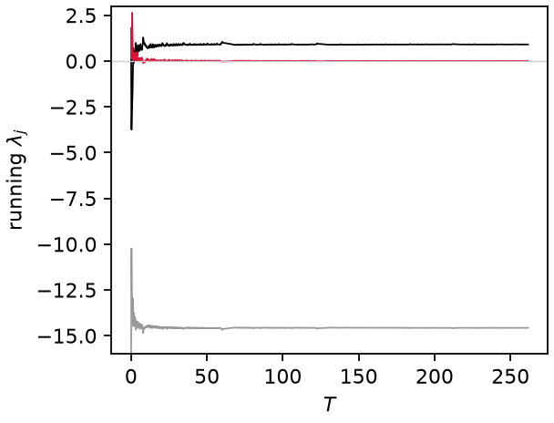
Running exponents of Lorenz63 converging to \([0.90,\ 0.00,\ -14.6]\).

Leading exponent from perturbation growth

Without any Jacobian (so it also works for discrete maps), leading_lyapunov evolves an ensemble of perturbed copies \(\psi + \delta_0 \mathbf{e}\) and fits the linear region of the mean log separation,

\[ \lambda_1 \approx \frac{d}{dt} \left\langle \ln \left\| \psi_\mathrm{pert}(t) - \psi_\mathrm{ref}(t) \right\| \right\rangle , \]

between the transient and the saturation plateau (automatic window; fit rejected if \(R^2 < 0.5\)).

Saturation guard. On a stable orbit, non-normal transient amplification can produce a large positive slope even though there is no chaos (thermoacoustic systems read \(\lambda_1 \sim 200\) this way). The fit is rejected when the separation saturates far below the attractor diameter while the tail has stopped growing:

\[ \text{sat} < 0.05 \cdot \mathrm{diam} \quad \text{and} \quad \text{tail slope} < 0.1\,\lambda_1 . \]

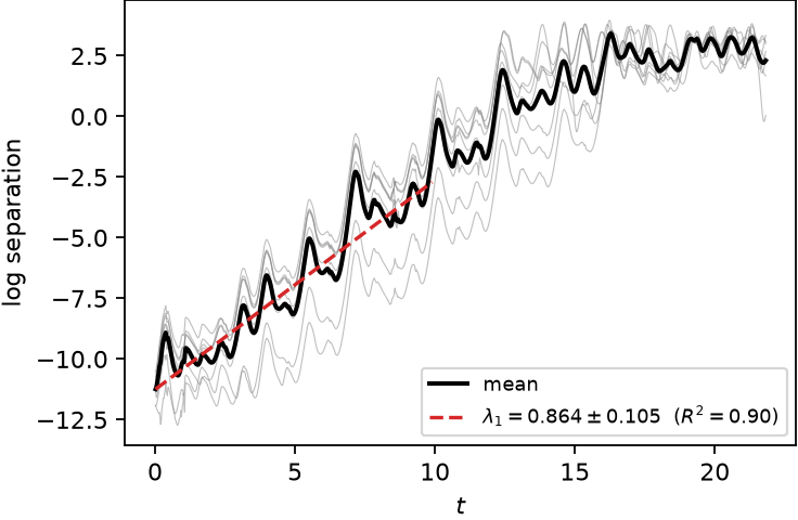
Perturbation-growth fit on Lorenz63: \(\lambda_1 = 0.86 \pm 0.11\) from the linear region of the mean log separation.

Data-only: Rosenstein estimator

When only a measured series is available, rosenstein_lyapunov applies the same idea to the delay embedding [Rosenstein et al. 1993]: each reference point \(\mathbf{y}_i\) is paired with its nearest neighbour \(\mathbf{y}_j\) at least one Theiler window \(w\) away in time (\(|i - j| > w\), with \(w\) the mean inter-maximum spacing, so pairs sample different orbits rather than adjacent samples of the same one), and the mean log divergence

\[ S(k) = \left\langle \ln \left\| \mathbf{y}_{i+k} - \mathbf{y}_{j+k} \right\| \right\rangle_{(i,j)} \]

is fitted over its linear window with the same machinery — and the same \(R^2\) and growth-range guards — as above, so periodic or noise-bound data returns nan rather than a spurious slope. Pairs are averaged in 8 blocks whose slope spread gives the quoted uncertainty. This is what DataSeries.analyze runs by default, letting measured data reach the chaotic label with no model at all:

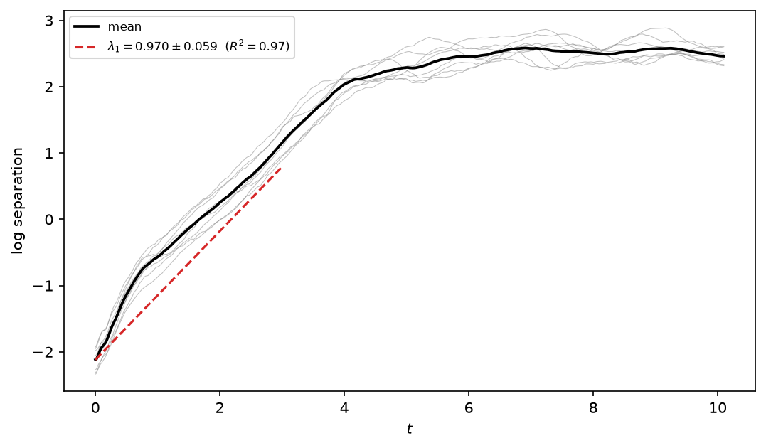
Lorenz63 from measurements only: \(\lambda_1 = 0.97 \pm 0.06\) against the true 0.906.

Kaplan–Yorke dimension

With the exponents sorted \(\lambda_1 \geq \lambda_2 \geq \dots\) and \(j\) the largest index with \(\sum_{i=1}^{j} \lambda_i \geq 0\),

\[ D_\mathrm{KY} = j + \frac{\sum_{i=1}^{j} \lambda_i}{\left| \lambda_{j+1} \right|} , \]

conjectured equal to the information dimension [Kaplan & Yorke 1979]. Shown as a text box on the delay-portrait panel.

References are collected on the theory overview.