Signal and attractor diagnostics

Qualitative fingerprints of the regime (PSD peaks, return map, recurrence, Poincaré section) and the quantitative attractor dimension \(D_2\).

Power spectral density

fun_PSD uses the one-sided FFT amplitude spectrum,

\[ \mathrm{PSD}(f_k) = \frac{2}{N} \left| \sum_{j=0}^{N-1} x_j\, e^{-2\pi i jk/N} \right| , \qquad f_k = \frac{k}{N\,\Delta t},\quad k < N/2 . \]

The classifier extracts the dominant peaks \(f_1, f_2, \dots\) from it (find_peaks with prominence thresholds) and tests their ratios for rationality.

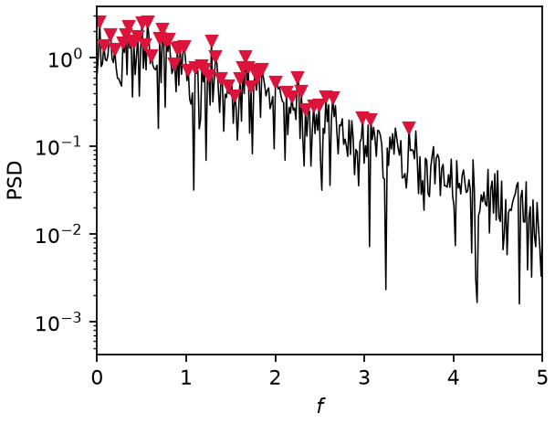
PSD of chaotic Lorenz63: broadband, with the dominant peaks the classifier extracts (markers).

First-return map and peak clusters

Successive local maxima of the signal form the return map \(x_{\max}(i+1)\) vs \(x_{\max}(i)\). A period-\(k\) orbit produces \(k\) tight clusters; count_peak_clusters counts maxima levels that differ by more than tol \(\times\) the signal range. This check outranks a positive perturbation-growth exponent in the classifier: \(k\) tight maxima levels over a long record are incompatible with chaos (see the decision tree).

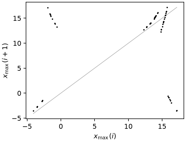
Return map of the Lorenz63 maxima: a continuum, not \(k\) tight clusters — chaos.

Recurrence plot

\[ R_{ij} = \Theta\!\left( \varepsilon - \left\| \mathbf{Y}_i - \mathbf{Y}_j \right\| \right), \]

with \(\Theta\) the Heaviside step and \(\varepsilon\) set to 10% of the maximum pairwise distance (retargeted to a fixed 10% recurrence rate when the density degenerates). Periodic dynamics give unbroken diagonals; quasiperiodic dynamics give diagonals of varying spacing; chaos gives short, broken diagonals [Eckmann et al. 1987].

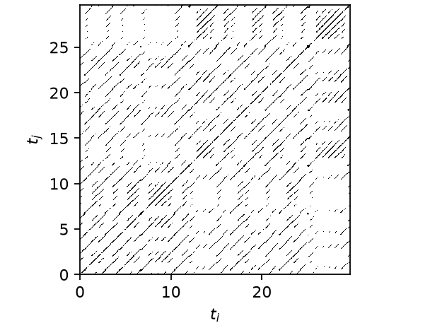
Recurrence plot of chaotic Lorenz63: short, broken diagonals.

Poincaré section

poincare_section intersects the 3-D delay embedding with the plane \(x(t + 2\zeta) = \text{level}\) (median by default), keeping upward crossings. Between bracketing samples \(i\) and \(i+1\) the crossing is linearly interpolated,

\[ \mathbf{P} = \mathbf{Y}_i + w\,(\mathbf{Y}_{i+1} - \mathbf{Y}_i), \qquad w = \frac{s_i}{s_i - s_{i+1}}, \]

where \(s = Y_3 - \text{level}\) is the signed distance to the plane. A limit cycle of period \(k\) appears as \(k\) points, a 2-torus as a closed loop, chaos as a fractal scatter.

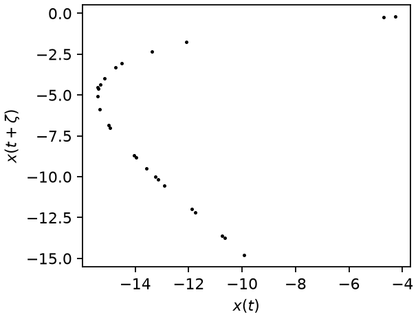
Poincaré section of chaotic Lorenz63: a fractal scatter.

Correlation dimension (Grassberger–Procaccia)

The correlation sum over pairs of points on the attractor (or section),

\[ C(r) = \frac{2}{n(n-1)} \sum_{i<j} \Theta\!\left( r - \left\| \mathbf{Y}_i - \mathbf{Y}_j \right\| \right) \;\propto\; r^{D_2} \quad (r \to 0), \]

gives \(D_2\) as the slope of \(\ln C\) vs \(\ln r\) fitted between the 2nd and 50th distance percentiles [Grassberger & Procaccia 1983]. For a \(k\)-torus \(D_2 \approx k\) on the attractor and \(\approx k-1\) on its Poincaré section — one of the three torus-dimension witnesses used in the worked example.

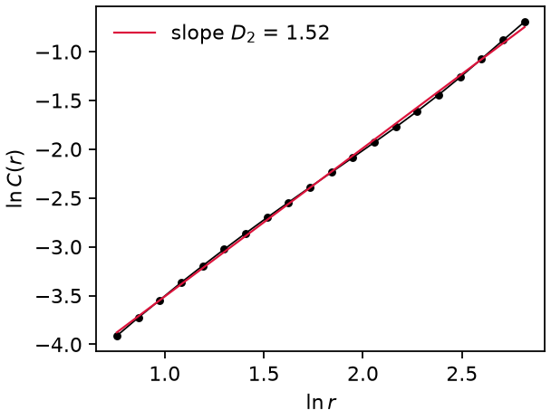
Correlation-sum fit for the Lorenz63 delay embedding: fractal \(D_2 = 1.5\).

References are collected on the theory overview.