Skip to content

romda

Real-time reduced-order modelling and bias-aware data assimilation.

romda is an open-source Python package for combining low-order forecast models with experimental data in real time. It provides:

  • Ensemble data assimilation — the ensemble Kalman filter (EnKF), the ensemble square-root Kalman filter (EnSRKF), and the regularized bias-aware EnKF (r-EnKF) of Nóvoa, Racca & Magri (2023), plus a linear Kalman filter.
  • Forecast models — physical low-order models (Rijke tube, azimuthal thermoacoustics, Van der Pol, Lorenz 63/96, Kuramoto–Sivashinsky) and data-driven reduced-order models (Echo State Networks and POD-ESN).
  • Bias estimators — interchangeable models of the (unknown) model bias: an ESN estimator, a constant (persistent) bias, and a zero-bias placeholder.
  • Modal decompositions — POD and spectral POD (Sieber 2016 and Towne 2018) with an sklearn-style fit / encode / decode interface.

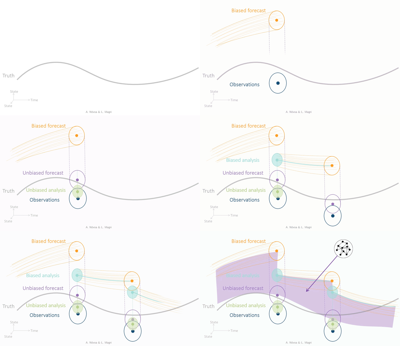
Real-time bias-aware DA

Real-time bias-aware data assimilation: forecast, bias correction, assimilation, and update.

Model choice trades off accuracy against computational cost — from cheap low-order physical models to expensive high-fidelity simulations, with data-driven reduced-order models in between:
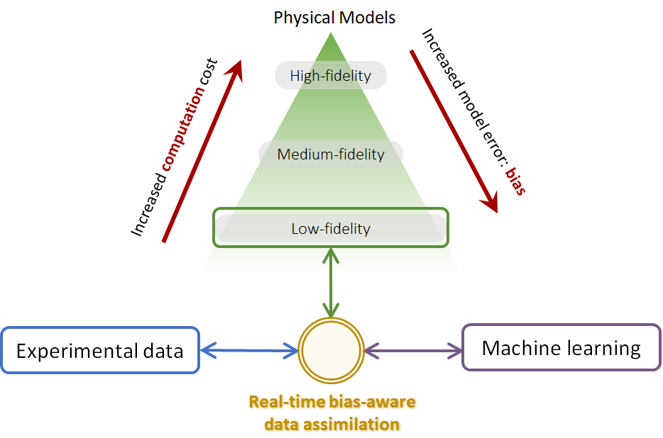
Model accuracy vs. computational cost

The source of model bias: physical models trade fidelity for speed.

Quick example

from romda.estimators.ensembles import rBA_EnKF
from romda.models.physical import VdP
from romda.bias_estimators import ConstantBias
from romda.observations import Observations

truth = Observations(model=VdP, t_start=0.6, t_stop=0.8, Nt_obs=30,
                      add_noise=True, manual_bias='linear')

ensemble = rBA_EnKF(parent_model=VdP(dt=truth.dt),
                     parent_bias=ConstantBias,
                     m=10, std_phi=0.1, std_alpha=dict(zeta=(40., 60.)))

for d, t_d in zip(truth.y_obs, truth.t_obs):
    ensemble.forecast_step(t_end=t_d)
    ensemble.analysis_step(d=d, Cdd=...)

Where to start

Citing

If you use romda in your research, please cite the relevant publications, in particular:

Nóvoa, A., Racca, A., & Magri, L. (2023). Inferring unknown unknowns: Regularized bias-aware ensemble Kalman filter. Computer Methods in Applied Mechanics and Engineering, 418, 116502.

Class Hierarchy

Table of Contents

  1. Models
  2. Estimator
  3. 2.1 Available Estimators
  4. Bias
  5. 3.1 Forecaster
  6. Observations

1. Models

Physical models — dynamodels.physical

All use IVPIntegrator (scipy solve_ivp) except KS.

Class Dim Key parameters Integrator
Lorenz63 3 rho, sigma, beta IVP
Lorenz96 Nx F, Nx IVP
VdP 2 beta, zeta, kappa, law, omega IVP
Annular 4 omega, nu, c2beta, kappa, epsilon IVP
KS Nx nu, L, Nx Discrete (ETDRK4)
Rijke 2Nm+Nc beta, tau, C1, C2, kappa IVP

Data-driven models — src/models/data_driven/

All use DiscreteIntegrator. The ML base classes EchoStateNetwork (from the external echostatenetwork package) and the Projector hierarchy (POD/SPOD, in src/models/data_driven/autoencoders/ — see Data-driven models) are mixed in via multiple inheritance.

Class Key parameters Notes
ESN_model N_units, rho, sigma_in, N_wash Inherits EchoStateNetwork; requires training data at init
POD_ESN N_modes, sensor_locations Inherits ESN_model + POD; sensor placement via QR
LinearModel F (transition matrix), Q_noise ψ_{t+1} = F @ ψ_t + noise

2. Estimator

File: src/estimators/__init__.py

Abstract base class (ABC) that wraps a Model and an optional Bias into a full DA loop. Provides the shared forecast_step() that advances both the model and the bias in time.

Key attributes: est_phi, est_alpha, est_bias, inflation_factor, num_DA_blind, num_SE_only

Key concrete methods: forecast_step(), _init_bias(), _MA() (applies measurement operator M)

Subclasses must implement: - analysis_step(d, Cdd) — Bayesian update given observation vector d and noise covariance Cdd

Estimator  (ABC)
├── EnsembleEstimator
│   ├── EnKF
│   ├── EnSRKF
│   └── rBA_EnKF
└── DeterministicEstimator
    └── KalmanFilter

The relationship between the three main classes — attributes, not subclasses:

Estimator instance
  .model  →  Model instance   (used for the forecast)
  .bias   →  Bias instance    (optional; None if bias-unaware)
             .forecaster  →  Model instance   (usually an ESN_model)

2.1 Available Estimators

Ensemble estimators — src/estimators/ensembles.py

EnsembleEstimator is the concrete intermediate base; leaf classes only implement _analysis_kernel(Af, d, Cdd).

Key attributes: m (ensemble size), std_phi, std_alpha, regularization_factor

Class Filter type Reference
EnKF Stochastic EnKF (perturbed observations) Evensen (2003)
EnSRKF Deterministic square-root EnKF Tippett et al. (2003)
rBA_EnKF Regularised bias-aware EnKF, weight γ Nóvoa & Magri (2022)

Deterministic estimators — src/estimators/deterministic.py

DeterministicEstimator owns the state mean ψ and covariance Cpp directly (no ensemble).

Class Notes
KalmanFilter Standard linear KF; propagates covariance with Jacobian F_jac

3. Bias

File: src/bias_estimators/bias.py

Base class for observation-bias estimators. Mixes in HistoryTracker. Wraps a forecaster model to produce bias corrections at each assimilation step.

Key attributes: innovation, dt, forecaster, Nq, N_dim, upsample, biased_observations

Subclasses must implement: - init_forecaster(**kwargs) — build/train the internal forecasting model - state_derivative() — return the Jacobian J = db/dy used by bias-aware filters

Bias
├── ESN_bias
└── ConstantBias
    └── NoBias
Class File Notes
ESN_bias src/bias_estimators/esn.py Correlation-based training; biased_observations = True; the workhorse
ConstantBias src/bias_estimators/constantbias.py Fixed bias estimate; NoBias subclass for bias-blind DA

3.1 Forecaster

The forecaster attribute of a Bias instance is a Model subclass — typically a data-driven model trained on the residual between observations and model output.

Bias instance
  .forecaster  →  Model instance   (usually ESN_model)

The forecaster is initialised inside init_forecaster() and stepped forward in sync with the main model during Estimator.forecast_step(). Its output is the predicted bias b(t), which enters the analysis step as a correction to the observation.


4. Observations

File: src/observations.py

Standalone class (no inheritance). Generates or loads ground-truth data, applies a configurable manual bias, adds noise, and exposes observation time indices for the DA loop.

Key attributes:

Attribute Description
y_true Clean biased truth signal (Nt, Nq, 1)
y_raw Noisy observed signal (Nt, Nq, 1)
b_true Applied bias (Nt, Nq, 1)
t_true Full time vector
y_obs, t_obs Observations at assimilation times
obs_idx Indices into t_true at which observations are taken
Nt_obs Subsampling rate (every Nt_obs steps)

Noise options (noise_type): 'gauss, add', 'gauss, mult', coloured noise variants.

Manual bias options (manual_bias): 'linear', 'periodic', 'time', 'cosine', or any callable f(y_true, t_true) -> (b, name).

Key method: plot_truth(case) — five-panel figure (raw, truth, PDF, PSD, difference).