TUTORIAL: Real-time data assimilation in a chaotic system

• The Ensemble Kalman filter (recap)
  • The EnKF update
• Test case: twin experiment on the Lorenz63 model
  • The true state and parameters
  • The observations
  • The ensemble
  • Data assimilation

Ensemble Kalman Filter: State & Parameter Estimation

Real-time data assimilation combines a numerical model with noisy observations to estimate the most likely state of a system. We use the Ensemble Kalman Filter (EnKF) — a sequential method that assimilates data on the fly, without storing or post-processing the full data history.

---

The EnKF fuses two sources of information:

1. Observations \(\mathbf{d} \sim \mathcal{N}(\mathbf{d}^\dagger, \mathbf{C}_{dd})\) — unbiased but noisy sensor measurements
2. Model forecast — a dynamical system propagating the state \(\boldsymbol{\phi}\) forward in time

\[\mathrm{d}\boldsymbol{\phi} = \mathcal{F}(\boldsymbol{\phi} + \boldsymbol{\epsilon}_\phi,\, \boldsymbol{\alpha} + \boldsymbol{\epsilon}_\alpha)\,\mathrm{d}t\]

such that the model prediction on the observations is \(\mathcal{M}(\boldsymbol{\phi}) \sim \mathcal{N}(\mathbf{d}^\dagger, \mathbf{C}_{\phi\phi})\), where \(\mathcal{M}\) is the measurement operator mappinf the state variables to the measurement space.

Since both sources are uncertain, we model all errors as Gaussian and seek the maximum a posteriori (MAP) estimate — the state \(\boldsymbol{\phi}^a\) that minimises:

\[\mathcal{J}(\boldsymbol{\phi}) = \underbrace{\|\boldsymbol{\phi} - \boldsymbol{\phi}^f\|^2_{(\mathbf{C}_{\phi\phi}^f)^{-1}}}_{\text{model penalty}} + \underbrace{\|\mathbf{d} - \mathcal{M}(\boldsymbol{\phi})\|^2_{\mathbf{C}_{dd}^{-1}}}_{\text{observation penalty}}\]

To estimate both state \(\boldsymbol{\phi}\) and parameters \(\boldsymbol{\alpha}\) simultaneously, we define an augmented state vector \(\boldsymbol{\psi} = [\boldsymbol{\phi};\, \boldsymbol{\alpha}; \mathcal{M}(\boldsymbol{\phi})]\), treating parameters as time-constant state variables:

\[\mathrm{d}\begin{bmatrix}\boldsymbol{\phi} \\ \boldsymbol{\alpha}\end{bmatrix} = \begin{bmatrix}\mathcal{F}(\boldsymbol{\phi} + \boldsymbol{\epsilon}_\phi,\, \boldsymbol{\alpha} + \boldsymbol{\epsilon}_\alpha) \\ \mathbf{0}\end{bmatrix}\mathrm{d}t\]

with this, the cost fucntion becomes

\[\mathcal{J}(\boldsymbol{\psi}) = \underbrace{\|\boldsymbol{\psi} - \boldsymbol{\psi}^f\|^2_{(\mathbf{C}_{\psi\psi}^f)^{-1}}}_{\text{model penalty}} + \underbrace{\|\mathbf{d} - \mathbf{M}\boldsymbol{\psi}\|^2_{\mathbf{C}_{dd}^{-1}}}_{\text{observation penalty}}\]

---

The EnKF Update

The EnKF propagates \(m\) ensemble members \(\boldsymbol{\psi}_j\) to approximate the forecast statistics (mean and covariance)

\[\bar{\boldsymbol{\psi}} = \frac{1}{m}\sum_{j=1}^m \boldsymbol{\psi}_j, \qquad \mathbf{C}_{\psi\psi} \approx \frac{1}{m-1}\sum_{j=1}^m (\boldsymbol{\psi}_j - \bar{\boldsymbol{\psi}})(\boldsymbol{\psi}_j - \bar{\boldsymbol{\psi}})^\top\]

When observations \(\mathbf{d}\) arrive, each member is updated as:

\[\boldsymbol{\psi}_j^\mathrm{a} = \boldsymbol{\psi}_j^\mathrm{f} + \mathbf{K}\left[\mathbf{d}_j - \mathbf{M}\boldsymbol{\psi}_j^\mathrm{f}\right]\]

where the Kalman gain \(\mathbf{K}\) optimally weights model and observation uncertainty:

\[\mathbf{K} = \mathbf{C}_{\psi\psi}^\mathrm{f}\,\mathbf{M}^\top\!\left(\mathbf{C}_{dd} + \mathbf{M}\mathbf{C}_{\psi\psi}^\mathrm{f}\mathbf{M}^\top\right)^{-1}\]

---

Test case: twin experiment on the Lorenz63 model

We validate the EnKF on the Lorenz 63 system — a canonical chaotic model:

\[\frac{\mathrm{d}x}{\mathrm{d}t} = \sigma(y - x), \qquad \frac{\mathrm{d}y}{\mathrm{d}t} = x(\rho - z) - y, \qquad \frac{\mathrm{d}z}{\mathrm{d}t} = xy - \beta z\]

with state \(\boldsymbol{\phi} = [x;\,y;\,z]\) and parameters \(\boldsymbol{\alpha} = [\sigma;\,\rho;\,\beta]\).

This system is chaotic at \(\boldsymbol{\alpha} = [10;\,28;\,8/3]\): two trajectories initialised 0.01% apart diverge exponentially, with a predictability horizon set by the Lyapunov time \(T_\lambda = 1/\lambda_\mathrm{max} \approx 1/0.91\). This makes it an ideal test for data assimilation — the EnKF must continuously correct the ensemble to track the true trajectory before it diverges.

We use a twin experiment: a synthetic truth \(\boldsymbol{\psi}^\dagger\) is integrated from the model, observations are generated as \(\mathbf{d} = \mathbf{M}\boldsymbol{\psi}^\dagger + \boldsymbol{\epsilon}_d\), and the EnKF attempts to recover both \(\boldsymbol{\phi}^\dagger\) and \(\boldsymbol{\alpha}^\dagger\) without access to the truth.

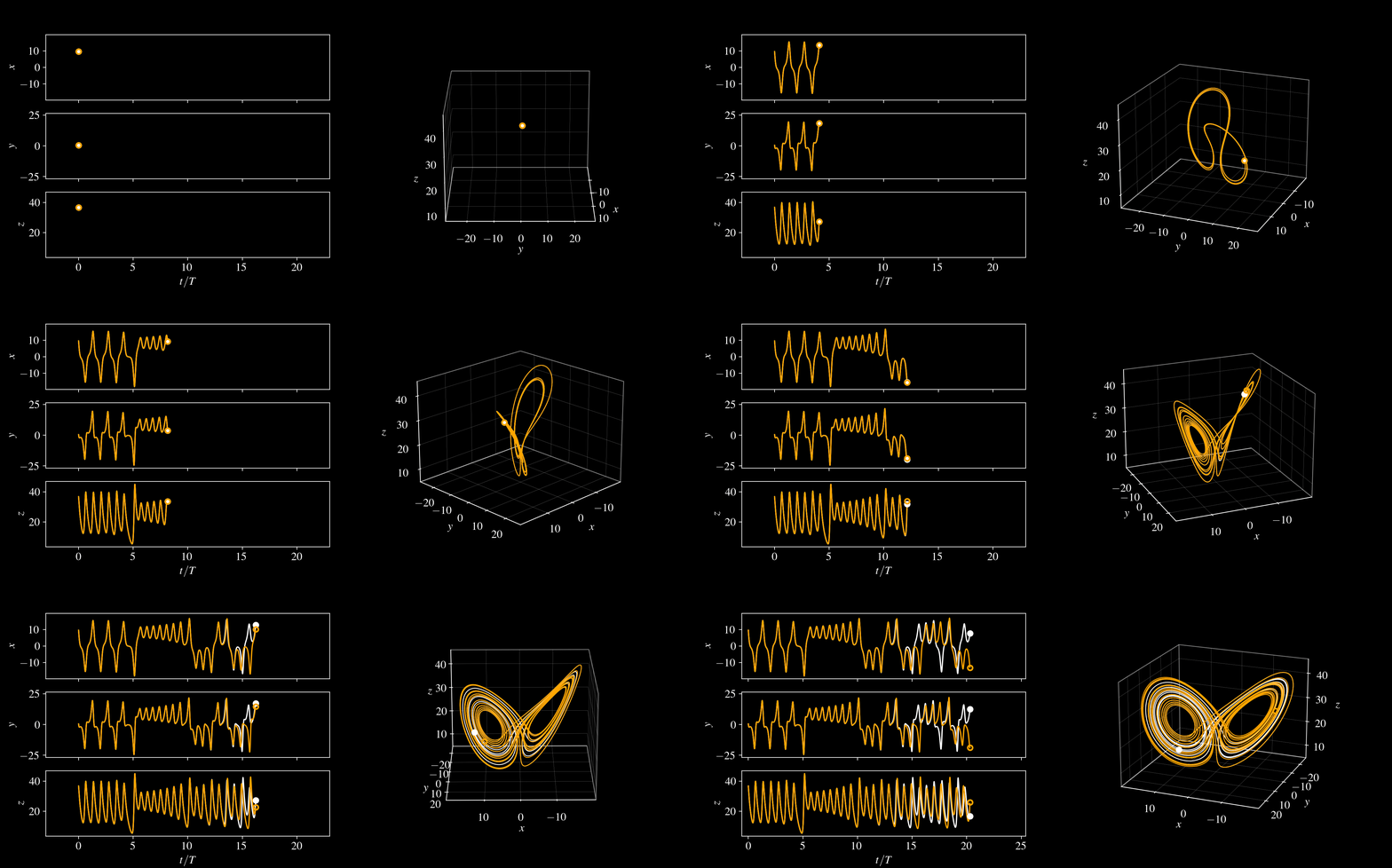
1) The true state and parameters

from romda.models.physical import Lorenz63
import numpy as np
rng = np.random.default_rng(0)

dt_t = 0.015
t_lyap = 0.9056 ** (-1)  # Lyapunov Time (inverse of maximal Lyapunov exponent)

true_params = dict(dt=dt_t,
                   rho=28.,
                   sigma=10.,
                   beta=8. / 3.,
                   psi0=rng.random(3)+10,
                   observe_dims=[0, 2]     # Select the dimensions to observe
                   )

# Initialize model
true_case = Lorenz63(**true_params)

# Forecast model
t_max = t_lyap * 100
psi, t = true_case.time_integrate(int(t_max / true_case.dt))
true_case.update_history(psi, t)

2) The observations

from romda.observations import Observations

# # Draw data points from raw data
dt_obs = t_lyap * .5  # time between analyses
Nt_obs = dt_obs // dt_t
t_start, t_stop = t_lyap * 10, t_lyap * 60 # start and end of assimilation


truth = Observations(model=true_case, 
                    t_start=t_start, 
                    t_stop=t_stop, 
                    Nt_obs=Nt_obs, 
                    add_noise=True,
                    noise_type='gauss, add',
                    noise_level=0.05,
                    )

Observations.plot_truth(truth)

3) Define the ensemble case

We create an ensemble with randomly generated states and parameters

from romda.estimators import EnSRKF, EnKF

alpha0 = dict(rho=(25., 35.),
              beta=(2, 4),
              sigma=(5,15))

ensemble = EnSRKF(parent_model=Lorenz63,      
                    dt=dt_t,             
                    m=50,               # Number of ensemble members
                    std_phi=0.2,        # Initial uncertainty in the state
                    std_alpha=alpha0,       # Initial uncertainty in the parameters
                    observe_dims=true_case.observe_dims
                    )

# Froecast ensemble without assimilation and visualize
ensemble.forecast_step(t_end=t_start-2*t_lyap, close=True)
ensemble.visualize_state(time_indices=[0,-1])

4) Apply data assimilation

We now have all the ingredients to start our data assimilation algorithm.

filter_ens = ensemble.copy()
filter_ens.inflation_factor = 1.02
# Define measurement error covariance matrix
var_d = 0.1* np.std(filter_ens.model.get_observable_hist(), axis=0).max(axis=-1)

Cdd = np.eye(filter_ens.model.Nq) * var_d**2

# ----------------------------------------------------------------------------

for d, t_d in zip(truth.y_obs, truth.t_obs):
    filter_ens.forecast_step(t_end=t_d)
    filter_ens.analysis_step(d=d, Cdd=Cdd)

# ----------------------------------------------------------------------------

#Forecast the ensemble further without assimilation
t_extra = filter_ens.model.hist_t[-1] + filter_ens.model.t_CR
filter_ens.forecast_step(t_extra, averaged=False, close=True)

print("number of assimilation steps: len(truth.t_obs) =", len(truth.t_obs))

filter_ens.visualize_history(plot_members=True, 
                             truth=truth, 
                             reference_t=t_lyap,
                             reference_a=true_case.alpha0)

# Visualize attractors
# from plot_results import plot_attractor
import matplotlib.pyplot as plt

case0 = true_case.copy()

filter_ens.model.close()
case1 = filter_ens.model.copy()

# Forecast both cases
Nt = 25 * int(t_lyap / case0.dt)
psi0, t0 = case0.time_integrate(Nt=Nt)
psi_ens, t1 = case1.time_integrate(Nt=Nt)

psi1 = psi_ens[:, :3, 0]
psi2 = psi_ens[:, :3, -1]

case0.visualize_attractor(psi_cases=[psi0, psi1, psi2])
plt.legend(['True system', 'Ensemble j = 0', 'Ensemble j = m'], frameon=False);

---

Exercise:

-How would you expect the solution to change if we decrease/increase the assimilation frequency?

-How would you expect the solution to change if we observe only part of the state?

---