TUTORIAL: Class Estimator
This tutorial introduces the Estimator class hierarchy and shows how to instantiate an estimator and run the forecast step.
The analysis step (Bayesian update with observations) is covered in 1_Introduction_to_real-time_DA/.
Contents 1. Class hierarchy 2. Instantiate an ensemble estimator 3. Inspecting the initial ensemble 4. Running the forecast step
1. Class hierarchy 
All estimators share a common abstract base Estimator (defined in estimators/__init__.py).
Every estimator exposes the same interface:
| Method | What it does |
|---|---|
forecast_step(t_end=...) |
Advance the model (and bias, if present) to a target time |
analysis_step(d, Cdd) |
Bayesian update — covered in 1_Introduction_to_real-time_DA/ |
visualize_history(...) |
Plot observable and parameter histories |
The concrete classes live in three sub-modules:
Estimator                          (abstract base — estimators/__init__.py)
├── EnsembleEstimator              (ensemble Kalman filter base, abstract)
│   ├── EnKF                       stochastic, perturbed-observation
│   ├── EnSRKF                     deterministic square-root
│   └── rBA_EnKF                   regularised bias-aware
├── DeterministicEstimator         (Kalman filter with explicit covariance)
│   └── KalmanFilter
The intermediate bases are abstract — they declare a kernel (_analysis_kernel, ...) holding the pure maths — so only the leaf classes can be instantiated.
The estimator owns:
- a Model — passed at construction time; the estimator handles instantiation, ensemble generation, and the forecast loop.
- a Bias model (optional) — stepped forward in sync with the model during forecast_step.
2. Instantiate an ensemble estimator 
EnsembleEstimator is abstract, so we instantiate one of its leaf filters — here the square-root EnSRKF (the choice does not matter for this tutorial, which only runs the forecast step).
Pass the model class (or an existing instance) as parent_model. All remaining keyword arguments are forwarded to the model constructor.
The estimator automatically:
1. Instantiates the model.
2. Generates the initial ensemble via model.init_ensemble(m, std_phi, std_alpha, ...).
3. Reads the measurement operator M from the model.
Key constructor arguments:
| Argument | Description |
|---|---|
parent_model |
Model class or instance to use for the forecast |
m |
Number of ensemble members |
std_phi |
Initial state perturbation (fractional std) |
std_alpha |
Initial parameter uncertainty — float or {name: (lo, hi)} |
parent_bias |
Optional Bias instance or class |
import numpy as np
import matplotlib.pyplot as plt

from romda.models.physical import Lorenz63
from romda.estimators.ensembles import EnSRKF


ensemble = EnSRKF(
    parent_model=Lorenz63,
    parent_bias=None,
    m=20,
    std_phi=0.5,                     # initial state spread
    std_alpha=dict(rho=(20., 30.)),  # rho drawn uniformly from [20, 30]
    observe_dims=[0, 1, 2],
    dt=0.02,
)

ensemble.print_parameters(indent=2)
EnSRKF
======
  m = 20
  est_phi = True
  est_alpha = ['rho']
  est_bias = False
  Na = 1
  regularization_factor = None
  inflation_factor = 1.0
  inflation_factor_rejection = 1.002
  === Model parameters: ===
    Model class: Lorenz63
    Nq = 3
    beta = 2.666667
    observe_dims = [0, 1, 2]
    rho = 28.000000
    sigma = 10.000000
    t_lyap = 1.090513
    Ensemble configuration: {'est_alpha': ['rho'], 'm': 20}
  === Bias parameters: ===
    No bias model.
3. Inspecting the initial ensemble 
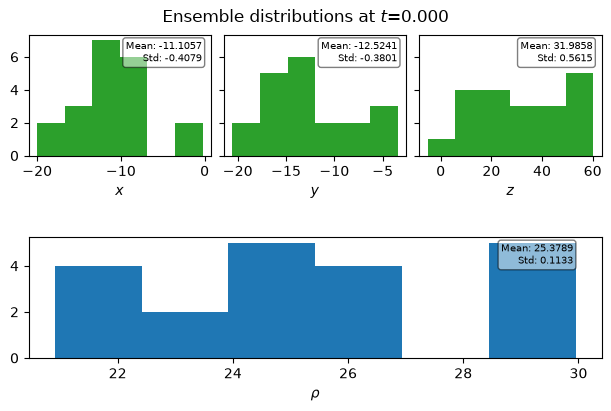
The ensemble state is stored in the model history (model.hist) with shape (Nt_history, Nphi + Na, m). At initialisation there is one time point.
The augmented state vector has Nphi physical state variables followed by Na estimated parameters.
psi0 = ensemble.current_state   # (Nphi, m)
print(f"Current state shape : {psi0.shape}")
print(f"Current time        : {ensemble.current_time}")
print(f"State mean          : {np.mean(psi0, axis=-1).round(3)}")
print(f"State std           : {np.std(psi0,  axis=-1).round(3)}")
Current state shape : (4, 20)
Current time        : 0.0
State mean          : [-11.106 -12.524  31.986  25.379]
State std           : [ 4.53   4.76  17.959  2.875]
ensemble.visualize_state()
4. Running the forecast step 
forecast_step(t_end=...) integrates the ensemble forward to t_end, appends the result to the model history, and (if a bias is attached) advances the bias model in sync.
estimator.forecast_step(t_end=t_target)
The number of integration steps is derived from t_end and model.dt automatically. The history grows with each call.
# Integrate forward for 5 Lyapunov times
t_end = ensemble.current_time + 10 * ensemble.model.t_lyap
ensemble.forecast_step(t_end=t_end)

print(f"History length : {len(ensemble.model.hist_t)} steps")
print(f"Time range     : {ensemble.model.hist_t[0]:.2f} --> {ensemble.model.hist_t[-1]:.2f}")
print(f"History shape  : {ensemble.model.hist.shape}  (Nt, Nphi+Na, m)")
Initializing multiprocessing pool for IVPIntegrator with m=20 and 20 pools.


History length : 546 steps
Time range     : 0.00 --> 10.90
History shape  : (546, 4, 20)  (Nt, Nphi+Na, m)
Visualising the forecast
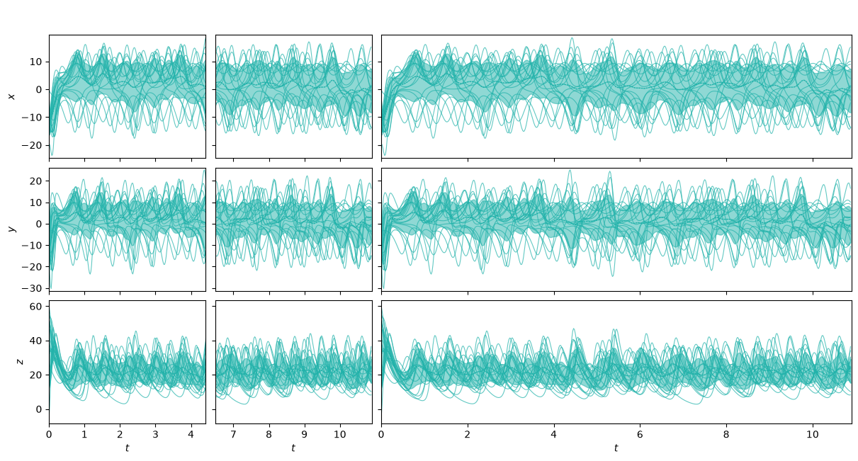
visualize_history plots the ensemble observable history. The three columns show an early window, a late window, and the full time axis.
ensemble.visualize_history(plot_members=True)
/storage0/anovoama/romda/src/estimators/ensembles.py:890: UserWarning: No artists with labels found to put in legend.  Note that artists whose label start with an underscore are ignored when legend() is called with no argument.
  fig1.legend(loc='center', bbox_to_anchor=(0.5, 1.05), ncol=6, frameon=False)