TUTORIAL: Real-time bias-aware data assimilation¶

What is bias-aware data assimilation?
- The source of bias: model accuracy vs computational cost
- Algorithmic view on bias-aware data assimilation
What is bias-aware data assimilation, a bit more technically?
The regularized ensemble Kalman filter
- Test case: van der Pol model with manually added bias

1. What is bias-aware data assimilation?¶

Real-time data assimilation combines quick estimates of a physical state from an numerical model with experimental data. In reality, numerical models are not a perfect representation of the physical quantity which we aim to predict because they typically rely on assumptions and simplifications for computational, i.e, they have an inherent model bias.

1.1. The source of bias: model accuracy vs computational cost¶

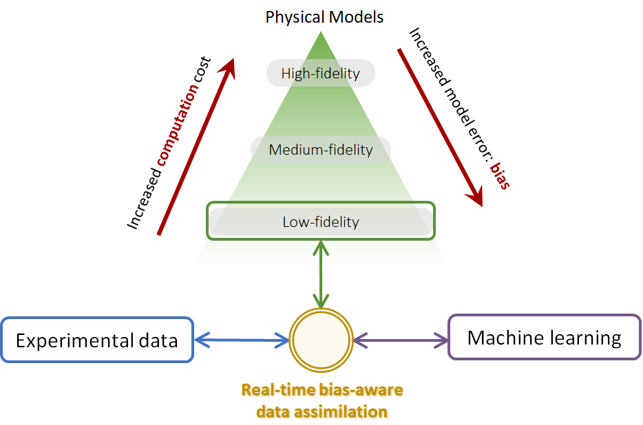
The choice of physical model plays a key role in the assimilation. Numerical models are mathematical representations of the processes that govern the behaviour of a physical system. For example, in weather forecasting, models simulate how the atmosphere evolves over time based on physical equations describing fluid dynamics, thermodynamics, etc. The more physical information we add to the model, the higher the accuracy of the model estimates. However, the computational requirements increase with the model complexity.

To perform real-time data assimilation we need quick estimates of the physical system. Thus, performing real-time high-fidelity modelling is not plausible in realistic scenarios. In order to apply real-time data assimilation to low-fidelity models, we must provide an estimate of the bias in the numerical model, i.e., the model error that we introduce when simplifying the physical equations.

1.2. Algorithmic view on bias-aware data assimilation¶

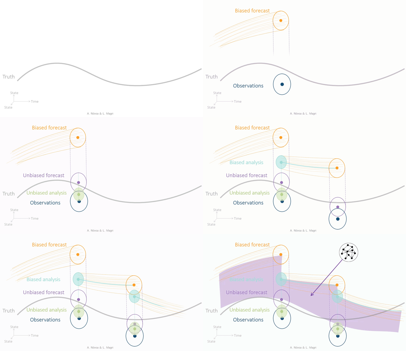
Algorithmically, we can summarize the bias-aware data assimilation process as: 1. Forecast: propagate the imperfect numerical model in time to provide a biased forecast when observation data become available. 2. Bias correction: provide an estimate the bias, and project the biased forecast into an unbiased forecast. 3. Assimilation: combine optimally the unbiased forecast with the observations. The direct assimilation results in an unbiased analysis, and the biased analysis is an indirect by-product of the assimilation. 4. Update: the biased analysis is the initial condition for the new forecast step.

2. What is bias-aware data assimilation, a bit more technically?¶

In this section, we revisit the formulation of the stochastic framework introduced in tutorial 11_ensemble-DA_intro.ipynb and we extend it to account for model biases.

2.1. Aleatoric and epistemic uncertainties¶

First, we discuss the statistical hypotheses on the aleatoric uncertainties. The aleatoric uncertainties contaminate the state and parameters as

\[ \boldsymbol{\phi} + \boldsymbol{\epsilon}_\phi = \boldsymbol{\phi}^\dagger, \quad \boldsymbol{\alpha} + \boldsymbol{\epsilon}_\alpha = \boldsymbol{\alpha}^\dagger, \]

where $\dagger$ indicates the true quantity (which is unknown). The aleatoric uncertainties are modelled as Gaussian distributions

\[ \boldsymbol{\epsilon}_\phi \sim \mathcal{N}( \mathbf{0}, \mathbf{C}_{\phi\phi} ), \quad \boldsymbol{\epsilon}_\alpha \sim \mathcal{N}( \mathbf{0}, \mathbf{C}_{\alpha\alpha} ), \]

where $\mathcal{N}( \mathbf{0}, \mathbf{C})$ is a normal distribution with zero mean and covariance $\mathbf{C}$. Second, we discuss model biases, which are epistemic uncertainties. The model bias is defined as the expected difference between the true observable and the model observable, i.e.,

\[ \mathbf{b} = \mathbf{d}^{\dagger} -\mathbb{E}( \mathbf{q}). \]

Hence, the bias-corrected model observable is

\[ \mathbf{y} = \mathbf{q} + \mathbf{b} + \boldsymbol{\epsilon}_q, \]

where $\boldsymbol{\epsilon}_q \sim \mathcal{N}( \mathbf{0}, \mathbf{C}_{qq})$. (If the model is unbiased, $\mathbf{d}^{\dagger} =\mathbb{E}( \mathbf{q})$.)

The final model equations, which define the first source of information on the system, are

\[ \begin{aligned} \left\{ \begin{array}{rcl} \mathrm{d} \boldsymbol{\phi}&=& \mathcal{F}\left( \boldsymbol{\phi+ \boldsymbol{\epsilon}_\phi, \alpha+ \boldsymbol{\epsilon}_\alpha} \right) \mathrm{d} t \\ \mathbf{y} &=& \mathcal{M}( \boldsymbol{\theta}, \boldsymbol{\phi}) + \mathbf{b}+ \boldsymbol{\epsilon}_q \end{array} \right. \end{aligned} \]

This set of equations is not closed because we need a model for the model bias. To infer it, we analyse the residuals between the forecast and the observations, which are also known as innovations

\[ \mathbf{i} = \mathbf{d} - \mathbf{q}. \]

As discussed in tutorial 11_ensemble-DA_intro.ipynb, the experimental data are affected by aleatoric noise such that $\mathbf{d} + \boldsymbol{\epsilon}_d = \mathbf{d}^{\dagger}$, where $\boldsymbol{\epsilon}_d \sim \mathcal{N}(\mathbf{0}, \mathbf{C}_{dd})$ and $\mathbf{C}_{dd}$ is a diagonal matrix with diagonal $\boldsymbol{\epsilon}_d$. With this, the expected value of the innovation is

\[ \mathbb{E}( \mathbf{i}) = \mathbf{b}, \]

i.e., the expected innovation is the model bias.

2.2. Augmented state-space formulation ¶

The augmented form of the state-space formulation of the model, accounting for th emodel bias, yields

\[ \begin{aligned} \left\{ \begin{array}{rcl} \mathrm{d}\begin{bmatrix} \boldsymbol{\phi}\\ \boldsymbol{\alpha}\\ \mathbf{q} \end{bmatrix} &=& \begin{bmatrix} \mathcal{F}( \boldsymbol{\phi}+ \boldsymbol{\epsilon}_\phi, \boldsymbol{\alpha}+ \boldsymbol{\epsilon}_\alpha)\\ \mathbf{0}_{N_\alpha}\\ \mathbf{0}_{N_q} \end{bmatrix} { \mathrm{d} t} \\ \mathbf{y} &=& \mathbf{q} + \mathbf{b} + \boldsymbol{\epsilon}_{q} \end{array} \right. \quad\leftrightarrow \quad \left\{ \begin{array}{rcl} \mathrm{d} \boldsymbol{\psi} &=& \mathbf{F}\left( \boldsymbol{\psi} + \boldsymbol{\epsilon}_\psi\right){ \mathrm{d} t} \\ \mathbf{y} &=& \mathbf{M} \boldsymbol{\psi} + \mathbf{b} + \boldsymbol{\epsilon}_{q} \end{array} \right. \end{aligned} \]

where $\mathbf{F}( \boldsymbol{\psi})$ and $\boldsymbol{\epsilon}_\psi$ are the augmented nonlinear operator and aleatoric uncertainties, respectively; $\mathbf{M} = \left[ \mathbf{0}~\big|~\mathbb{I}_{N_q}\right]$ is the linear measurement operator; and $\mathbf{0}_{N_\alpha}$ and $\mathbf{0}_{N_q}$ are vectors of zeros (because the parameters are constant in time, and $\mathbf{q}$ is not integrated in time but it is only computed at the analysis step).

2.3. Model bias in a stochastic ensemble framework ¶

The underlying assumption of ensemble methods is that the ensemble is Gaussian distributed, i.e, $\boldsymbol{\psi}_j\sim\mathcal{N}(\bar{ \boldsymbol{\psi}}, \mathbf{C}_{\psi\psi})$. Within an ensemble framework, we approximate the model bias with the ensemble statistics

\[ \begin{aligned} \mathbf{b} &\approx \mathbf{d}^{\dagger} - \mathbf{M}\bar{ \boldsymbol{\psi}}, \end{aligned} \]

Hence, the innovation of the ensemble mean can be approximated as

\[ \bar{ \mathbf{i}} = \mathbf{d} - \mathbf{M}\bar{ \boldsymbol{\psi}} \approx \mathbf{b}. \]

Exercise¶

How does the definition of the innovaition change is we did not assume unbiased observations? This is, $\mathbb{E}(\mathbf{d}) \neq \mathbf{d}^{\dagger}$.

2.4. How do we estimate the bias in time?¶

The model bias is defined as is the expected difference between the true observable and the model observable. Therefore, it is unknown a priori (colloquially, it is an unknown unknown). The model bias may be a function of the physical state, the environment or even a function of time.

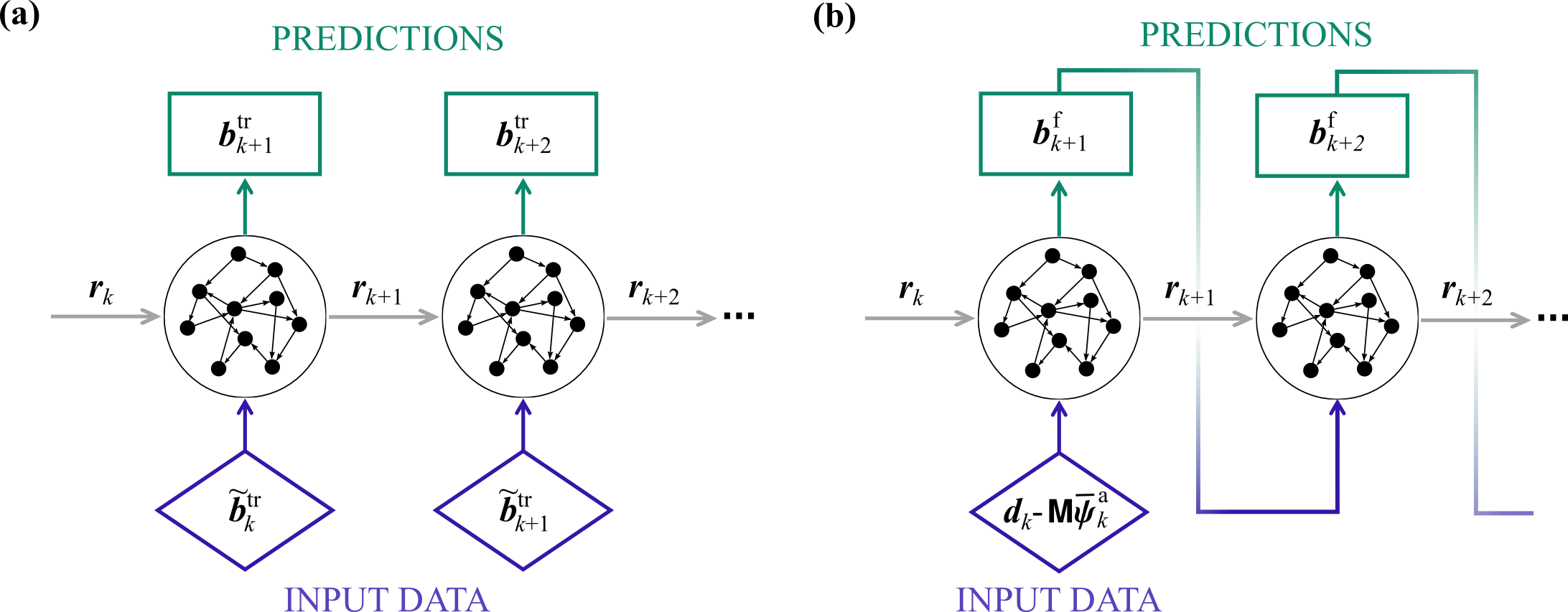
Recent advances in machine learning for data-driven modelling allow us to develop surrogate models of dynamical systems using neural networks. This is, we can use a neural network to estimate the bias of the low-order numerical models. Specifically, we employ an echo state network (ESN) to infer the model bias. ESNs are suitable for real-time data assimilation because 1. they are recurrent neural networks, i.e., they are designed to learn temporal dynamics in data; 2. they are based on reservoir computing, hence they are universal approximators; 3. they are general nonlinear autoregressive models; and 4. training an ESN consists of solving a linear regression problem, which provides a global minimum without backpropagation.

The architecture of the model bias estimation by ESN is illustrated below. The network runs in open loop only during training (left), whilst during operation the ESN performs one open-loop step when observations are available and then runs autonomously in closed loop until the next analysis (right).

3. The bias-regularized ensemble Kalman filter¶

The objective function in a bias-regularized data assimilation framework contains three norms

\[ \begin{aligned} \mathcal{J}( \boldsymbol{\psi}_j) = &\left\| \boldsymbol{\psi}_j- \boldsymbol{\psi}_j^\mathrm{f}\right\|^2_{ \mathbf{C}^{\mathrm{f}^{-1}}_{\psi\psi}} + \left\|{ \mathbf{y}}_j- \mathbf{d}_j\right\|^2_{\mathbf{C}^{-1}_{dd}}+\gamma\left\| \mathbf{b}_j\right\|^2_{ \mathbf{C}^{-1}_{bb}}, \quad \mathrm{for} \quad j=0,\dots,m-1 \end{aligned} \]

where the superscript 'f' indicates 'forecast'; the operator $\left\|\cdot\right\|^2_{ \mathbf{C}^{-1}}$ is the $L_2$-norm weighted by the semi-positive definite matrix ${ \mathbf{C}^{-1}}$; $\gamma\geq0$ is a user-defined bias regularization factor; and $\mathbf{b}_j$ is the model bias of each ensemble member. For simplicity, we define the bias in the ensemble mean, such that $\mathbf{b}_j = \mathbf{b}$ for all $j$. From left to right, the norms on the right-hand-side of the cost fuction measure 1. the spread of the ensemble prediction, 2. the distance between the bias-corrected estimate and the observables, and 3. the model bias norm.

The analytical solution of the bias-regularized ensemble Kalman filter (r-EnKF), which globally minimizes the cost function with respect to $\boldsymbol{\psi}_j$, is

\[ \begin{aligned} \boldsymbol{\psi}_j^\mathrm{a} &= \boldsymbol{\psi}_j^\mathrm{f} + \mathbf{K}_\mathrm{r} \left[\left(\mathbb{I}+ \mathbf{J}\right)^\mathrm{T}\left( \mathbf{d}_j - \mathbf{y}_j^\mathrm{f}\right) - \gamma \mathbf{C}_{dd} \mathbf{C}^{-1}_{bb} \mathbf{J}^\mathrm{T} \mathbf{b}^\mathrm{f}\right], \quad j=0,\dots,m-1 \end{aligned} \]

with

\[ \begin{aligned} \mathbf{K}_\mathrm{r} = \mathbf{C}_{\psi\psi}^\mathrm{f} \mathbf{M}^\mathrm{T}\left[ \mathbf{C}_{dd} + (\mathbb{I}+ \mathbf{J})^\mathrm{T}(\mathbb{I}+ \mathbf{J}) \mathbf{M} \mathbf{C}_{\psi\psi}^\mathrm{f} \mathbf{M}^\mathrm{T} + \gamma \mathbf{C}_{dd} \mathbf{C}^{-1}_{bb} { \mathbf{J}}^\mathrm{T}\mathbf{J} \mathbf{M} \mathbf{C}_{\psi\psi}^\mathrm{f} \mathbf{M}^\mathrm{T}\right]^{-1}, \end{aligned} \]

where 'a' stands for 'analysis', i.e, the optimal state of the assimilation; $\mathbf{K}_\mathrm{r}$ is the regularized Kalman gain matrix; and $\mathbf{J} = \mathrm{d} \mathbf{b}/ \mathrm{d} \mathbf{M} \boldsymbol{\psi}$ is the Jacobian of the bias estimator. We prescribe $\mathbf{C}_{dd} = \mathbf{C}_{bb}$ because the model bias is defined in the observable space. We use $\gamma$ to tune the norm of the bias. The optimal state and parameters are

\[ \begin{aligned} \begin{bmatrix} \boldsymbol{\phi}_j^\mathrm{a}\\ \boldsymbol{\alpha}_j^\mathrm{a} \end{bmatrix} = \begin{bmatrix} \boldsymbol{\phi}_j^\mathrm{f}\\ \boldsymbol{\alpha}_j^\mathrm{f} \end{bmatrix} + \overbrace{ \begin{bmatrix} \mathbf{C}_{\phi q}^\mathrm{f}\\ \mathbf{C}_{\alpha q}^\mathrm{f} \end{bmatrix} \left\{ \mathbf{C}_{dd}+(\mathbb{I}+ \mathbf{J})^\mathrm{T} (\mathbb{I}+ \mathbf{J}) \mathbf{C}_{qq}^\mathrm{f}+\gamma { \mathbf{J}}^\mathrm{T}\mathbf{J} \mathbf{C}_{qq}^\mathrm{f}\right\}^{-1} }^\mathrm{Regularized\, Kalman \, gain,\, \mathbf{K}_\mathrm{r}} \Big[\left(\mathbb{I}+\mathbf{J}\right)^\mathrm{T}\left(\mathbf{d}_j - \mathbf{y}_j^\mathrm{f}\right)- \gamma \mathbf{J}^\mathrm{T} \mathbf{b}^\mathrm{f}\Big] \end{aligned} \]

The r-EnKF defines a `good' analysis from a biased model if the unbiased state $\mathbf{y}$ matches the truth, and the model bias $\mathbf{b}$ is small relative to the truth. The underlying assumptions of this work are that (i) our low-order model is qualitatively accurate such that the model bias $\mathbf{b}^\mathrm{f}$ has a small norm; and (ii) the sensors are properly calibrated.

Exercise¶

Proof that in the limiting case when the assimilation framework is unbiased, the r-EnKF becomes the bias-unregularized EnKF, which we discussed in the previous tutorials.

rBA_EnKF(Af, d, Cdd, Cbb, k, M, b, J): """ Bias-aware Ensemble Kalman Filter. Inputs: Af: forecast ensemble at time t (augmented with Y) [N x m] d: observation at time t [Nq x 1] Cdd: observation error covariance matrix [Nq x Nq] Cbb: bias covariance matrix [Nq x Nq] k: bias penalisation factor M: matrix mapping from state to observation space [Nq x N] b: bias of the forecast observables (Y = MAf + B) [Nq x 1] J: derivative of the bias with respect to the input [Nq x Nq] Returns: Aa: analysis ensemble (or Af is Aa is not real) """ m = np.size(Af, 1) Nq = len(d) Iq = np.eye(Nq) # Mean and deviations of the ensemble Psi_f = Af - np.mean(Af, 1, keepdims=True) S = np.dot(M, Psi_f) Q = np.dot(M, Af) # Create an ensemble of observations D = rng.multivariate_normal(d, Cdd, m).transpose() # Correct the model estimate with the bias Y = Q + b Cqq = np.dot(S, S.T) # covariance of observations M Psi_f Psi_f.T M.T if np.array_equiv(Cdd, Cbb): CdWb = Iq else: CdWb = np.dot(Cdd, la.inv(Cbb)) Cinv = (m - 1) * Cdd + np.dot(np.dot(Iq + J.T, Iq + J), Cqq) + k * np.dot(CdWb, np.dot(np.dot(J.T, J), Cqq)) K = np.dot(Psi_f, np.dot(S.T, la.inv(Cinv))) Aa = Af + np.dot(K, np.dot(Iq + J.T, D - Y) - k * np.dot(CdWb, np.dot(J.T, np.repeat(b, m, axis=1)))) return Aa

import scipy.linalg as la import numpy as np rng = np.random.default_rng(0)

3.1. Test case: van der Pol model with manually added bias¶

from romda.observations import Observations from romda.models.physical import VdP import numpy as np rng = np.random.default_rng(0) # The manual bias is a function of state and/or time def manual_bias(y, t): # Linear function of the state # return .2 * y + .3 * np.max(y, axis=0), 'linear' # Periodic function of the state return 0.5 * np.max(y, axis=0) * np.cos(2 * y / np.max(y, axis=0)), 'periodic' # Time-varying bias # return .4 * y * np.sin((np.expand_dims(t, -1) * np.pi * 2) ** 2), 'time' # return 0.*y, 'None' truth = Observations(model=VdP, t_min=0.5, t_start=0.6, t_stop=.8, psi0=np.array([2., 1.]), t_max=1.5, Nt_obs=10, add_noise=True, noise_type='gauss, add', noise_level=0.1, manual_bias=manual_bias, include_washout=0 ) Observations.plot_truth(truth, f_max=1000)

...Applying user-defined manual bias ...Adding noise: gauss, add with level 0.1. OK: Observations initialized.

from romda.utils import set_working_directories results_folder = set_working_directories('VdP_bias')[1]

ii. Define ensemble¶

from romda.estimators.ensembles import EnSRKF, EnKF, rBA_EnKF alpha0 = dict( zeta=(40, 50.), # beta=(50, 80), # kappa=(3, 5), ) forecast_model = VdP(dt=truth.dt,) # alpha0 = dict() ensemble = rBA_EnKF(results_folder=results_folder, # Folder to save results # Data assimilation parameters regularization_factor=1., inflation_factor=1.0, # Model parameters parent_model=forecast_model, m=10, # Number of ensemble members std_phi=1.5, # Initial uncertainty in the state std_alpha=alpha0, # Initial uncertainty in the parameters alpha_distr='uniform', )

OK: Initialised VdP_default_ensemble_m10 history shape=(1, 3, 10) t=[0.]

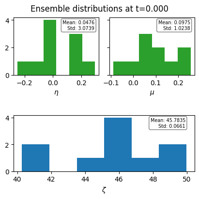
ensemble.visualize_state()

iii. Train an ESN to model the model bias¶

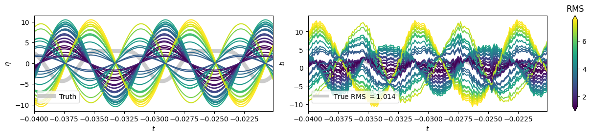
The procedure is the following: - Initialise ESN Bias class object - Create synthetic bias to use as training data - Train the ESN - Create washout data

from romda.bias_estimators import ESN_bias import matplotlib.pyplot as plt plt.close('all') training_data_filename = f'{results_folder}/Tutorial_13_{truth.name_bias}_bias_noise{truth.noise_level}_stda32' # Filename to save training data and results training_data_filename += '99' # Add suffix to distinguish training data with different options bias_estimator = ESN_bias(rom=ensemble.model, training_data_filename=training_data_filename, reference_data=truth, # Other options biased_observations=False, correlation_based_training=1, augment_data=2, add_noise=False, perform_test=True, t_train=ensemble.model.t_CR*10, t_val=ensemble.model.t_CR*1., t_test=ensemble.model.t_CR, upsample=5, N_units=50, N_wash=30, N_func_evals=20, N_folds=4, N_grid=4, rho_range=(0.7, 1.), sigma_in_range=(-5, 0), tikh_range=[1e-12, 1e-10, 1e-8], norm_method='range', random_initialization=True, plot_training=False, force_retrain=True, N_ens=25, L=25, std_alpha= dict(zeta=(40, 50.), beta=(50, 80), kappa=(3, 5)), std_phi=1. ) # Initialize bias model

✓ Found matching config: 13b1c7dac32883ba Configuration loaded from ...config/esn_configs/13b1c7dac32883ba/esn_config.yaml

from matplotlib.colors import Normalize import matplotlib.pyplot as plt def plot_train_data(truth, bias_data, t_CR): L, _, _ = bias_data['data'].shape Nt = int(t_CR / truth.dt) Nq = truth.y_true.shape[1] # Build a common valid time window and select the segment before first observation. n_common = min( len(truth.t_true), truth.y_true.shape[0], truth.b_true.shape[0], bias_data['y_model'].shape[0], bias_data['data'].shape[1], ) t0 = bias_data['y_model'].shape[0] yt = truth.y_raw[-t0:-t0+Nt] bt = truth.b_true[-t0:-t0+Nt] tt = truth.t_true[-t0:-t0+Nt] yr = bias_data['y_model'][:Nt].transpose(2, 0, 1) br = bias_data['data'][:, :Nt, :Nq] if len(tt) == 0: raise ValueError('Selected plotting window is empty. Check t_CR and training_data dimensions.') RS = [] for ii in range(L): RS.append(np.linalg.norm(br[ii][:, 0]) / np.sqrt(len(yt))) RS = np.asarray(RS, dtype=float) true_RMS = np.linalg.norm(bt[:, 0]) / np.sqrt(len(yt)) # Plot training data (single row) -------------------------- fig = plt.figure(figsize =[12, 2.7], layout='constrained') axs = fig.subplots(1, 2) # Robust color mapping: clip outliers; if RMS are nearly equal, force distinct member colors. if np.ptp(RS) < 1e-12: color_values = np.linspace(0.0, 1.0, L) norm = Normalize(vmin=0.0, vmax=1.0) cmap = plt.cm.ScalarMappable(norm=norm, cmap=plt.get_cmap('viridis')) cbar_extend = 'neither' cbar_title = 'Member' else: lo, hi = np.percentile(RS, [5, 95]) if np.isclose(lo, hi): lo = float(np.min(RS)) hi = float(np.max(RS)) color_values = np.clip(RS, lo, hi) norm = Normalize(vmin=float(lo), vmax=float(hi)) cmap = plt.cm.ScalarMappable(norm=norm, cmap=plt.get_cmap('viridis')) cbar_extend = 'both' cbar_title = '$\\mathrm{RMS}$' xlim = [tt[0], tt[-1]] axs[0].plot(tt, yt[:, 0], color='silver', linewidth=6, alpha=.8) axs[1].plot(tt, bt[:, 0], color='silver', linewidth=4, alpha=.8) for ii in range(L): clr = cmap.to_rgba(color_values[ii]) axs[0].plot(tt, yr[ii][:, 0], color=clr, alpha=0.7) axs[1].plot(tt, br[ii][:, 0], color=clr, alpha=0.7) axs[0].legend(['Truth'], bbox_to_anchor=(0., 0.25), loc='upper left') axs[1].legend(['True RMS $={0:.3f}$'.format(true_RMS)], bbox_to_anchor=(0., 0.25), loc='upper left') axs[0].set(xlabel='$t$', ylabel='$\\eta$', xlim=xlim) axs[1].set(xlabel='$t$', ylabel='$b$', xlim=xlim) clb = fig.colorbar(cmap, ax=axs, orientation='vertical', extend=cbar_extend) clb.ax.set_title(cbar_title)

from romda.bias_estimators.aux import plot_train_data import numpy as np # training_data_filename = f'{results_folder}/Tutorial_13_{truth.name_bias}_bias_noise{truth.noise_level}' # Filename to save training data and results training_data = np.load(f'{training_data_filename}', allow_pickle=True) plot_train_data(truth, training_data, t_CR=0.02) print(training_data['data'].shape)

(50, 4800, 1)

iv. Run DA cycle¶

# Observation covariance matrix (consistent with main branch) std_obs = 0.01 Cdd = np.diag(std_obs * np.ones(ensemble.model.Nq)) * np.max(abs(truth.y_obs), axis=0) ** 2

filter_ens = ensemble.copy() filter_ens.bias = bias_estimator.copy() filter_ens.bias.bayesian_update = True filter_ens.regularization_factor = 1. filter_ens.inflation_factor_rejection = 1. filter_ens.num_bias_blind = 0 ii = -1 J = [] inn = [] inn_t = [] for d, t_d in zip(truth.y_obs, truth.t_obs): ii += 1 if ii % 4 == 0: print(f'Assimilation step {ii}, time {t_d:.3f}') filter_ens.forecast_step(t_end=t_d.copy()) # J.append(filter_ens.bias.state_derivative()) y = filter_ens.model.get_observables() # bias_state = filter_ens.bias.update_state_from_innovation(d - y) # Innovation is observation minus analysis inn.append(d - y) inn_t.append(t_d) # filter_ens.bias.update_history(bias_state, # Innovation (observation - analysis) # filter_ens.current_time, modify_saved_states=True) b = filter_ens.bias.get_innovations(filter_ens.bias.current_bias) print('shapes', d.shape, y.shape, inn[-1].shape) print('bias', b.shape) # raise NotImplementedError('Bias update not implemented yet. This is a placeholder for the bias update step, which will be added in future iterations of the code. The bias update will involve using the innovation (observation minus analysis) to update the bias state, and then applying this updated bias state to correct the forecast before the analysis step.') filter_ens.analysis_step(d=d.copy(), Cdd=Cdd.copy()) if ii > 100: break

Assimilation step 0, time 0.100 Initializing multiprocessing pool for IVPIntegrator with m=10 and 10 pools. shapes (1,) (1, 10) (1, 10) bias (1, 1, 25) Non-physical analysis: 1/1 --------------------------------------------------------------------------- AttributeError Traceback (most recent call last) Cell In[10], line 32 29 print('bias', b.shape) 30 # raise NotImplementedError('Bias update not implemented yet. This is a placeholder for the bias update step, which will be added in future iterations of the code. The bias update will involve using the innovation (observation minus analysis) to update the bias state, and then applying this updated bias state to correct the forecast before the analysis step.') ---> 32 filter_ens.analysis_step(d=d.copy(), Cdd=Cdd.copy()) 34 if ii > 100: 35 break File ~/codes/real-time-bias-aware-DA/src/estimators/ensembles.py:318, in EnsembleEstimator.analysis_step(self, d, Cdd, return_analysis) 316 # ── Update model history ───────────────────────────────────────────── 317 state_size = self.model.Nphi + self.Na --> 318 self.update_history( 319 Aa[:state_size, :], 320 self.current_time, 321 modify_saved_states=True, 322 ) 323 self.assimilated_data = (d, self.current_time) 325 if return_analysis: File ~/codes/real-time-bias-aware-DA/src/estimators/ensembles.py:256, in EnsembleEstimator.update_history(self, psi, t, b, modify_saved_states, reset) 254 self.model.update_history(psi, t, reset=reset, modify_saved_states=modify_saved_states) 255 if self.bias is not None: --> 256 self.bias.update_history(b, t, reset=reset, modify_saved_states=modify_saved_states) File ~/codes/real-time-bias-aware-DA/src/bias.py:299, in Bias.update_history(self, state, t, reset, modify_saved_states, **kwargs) 298 def update_history(self, state, t=None, reset=False, modify_saved_states=False, **kwargs): --> 299 state = self._format_state(state) # Ensure shape (nt, nstate, nens) 301 # Ensure time array matches nt 302 if t is None: File ~/codes/real-time-bias-aware-DA/src/bias.py:207, in Bias._format_state(self, b) 203 def _format_state(self, b): 204 """ 205 Ensure b has shape (nt, nb, nens) 206 """ --> 207 if b.ndim == 3: 208 return b # already (nt, nb, nens) 209 elif b.ndim == 1: AttributeError: 'NoneType' object has no attribute 'ndim'

plt.plot(filter_ens.bias.hist_t, filter_ens.bias.get_innovations(state=filter_ens.bias.hist)[:, 0], label='Bias estimate') inn_array = np.array(inn)[:, 0] conv_inn = inn_array - np.mean(inn_array, axis=-1, keepdims=True) # Centered innovations (obs_dim, Nens) cov_inn = np.cov(conv_inn, rowvar=True) # Full covariance of innovations (obs_dim, obs_dim) cov_inn_2 = np.cov(conv_inn, rowvar=True) # Full covariance of centered innovations (obs_dim, obs_dim) plt.errorbar(np.array(inn_t), np.mean(inn_array, axis=-1), yerr=np.std(conv_inn, axis=-1), label='Observations', c='r', ls='') plt.errorbar(np.array(inn_t), np.mean(inn_array, axis=-1), yerr=np.std(cov_inn_2, axis=-1), label='Observations', c='b', ls='', alpha=0.5) plt.xlim(0.15, 0.2)

--------------------------------------------------------------------------- AxisError Traceback (most recent call last) Cell In[11], line 10 7 cov_inn_2 = np.cov(conv_inn, rowvar=True) # Full covariance of centered innovations (obs_dim, obs_dim) 9 plt.errorbar(np.array(inn_t), np.mean(inn_array, axis=-1), yerr=np.std(conv_inn, axis=-1), label='Observations', c='r', ls='') ---> 10 plt.errorbar(np.array(inn_t), np.mean(inn_array, axis=-1), yerr=np.std(cov_inn_2, axis=-1), label='Observations', c='b', ls='', alpha=0.5) 12 plt.xlim(0.15, 0.2) File ~/codes/real-time-bias-aware-DA/.venv/lib/python3.14/site-packages/numpy/_core/fromnumeric.py:4028, in std(a, axis, dtype, out, ddof, keepdims, where, mean, correction) 4025 else: 4026 return std(axis=axis, dtype=dtype, out=out, ddof=ddof, **kwargs) -> 4028 return _methods._std(a, axis=axis, dtype=dtype, out=out, ddof=ddof, 4029 **kwargs) File ~/codes/real-time-bias-aware-DA/.venv/lib/python3.14/site-packages/numpy/_core/_methods.py:219, in _std(a, axis, dtype, out, ddof, keepdims, where, mean) 217 def _std(a, axis=None, dtype=None, out=None, ddof=0, keepdims=False, *, 218 where=True, mean=None): --> 219 ret = _var(a, axis=axis, dtype=dtype, out=out, ddof=ddof, 220 keepdims=keepdims, where=where, mean=mean) 222 if isinstance(ret, mu.ndarray): 223 ret = um.sqrt(ret, out=ret) File ~/codes/real-time-bias-aware-DA/.venv/lib/python3.14/site-packages/numpy/_core/_methods.py:152, in _var(a, axis, dtype, out, ddof, keepdims, where, mean) 148 def _var(a, axis=None, dtype=None, out=None, ddof=0, keepdims=False, *, 149 where=True, mean=None): 150 arr = asanyarray(a) --> 152 rcount = _count_reduce_items(arr, axis, keepdims=keepdims, where=where) 153 # Make this warning show up on top. 154 if ddof >= rcount if where is True else umr_any(ddof >= rcount, axis=None): File ~/codes/real-time-bias-aware-DA/.venv/lib/python3.14/site-packages/numpy/_core/_methods.py:83, in _count_reduce_items(arr, axis, keepdims, where) 81 items = 1 82 for ax in axis: ---> 83 items *= arr.shape[mu.normalize_axis_index(ax, arr.ndim)] 84 items = nt.intp(items) 85 else: 86 # TODO: Optimize case when `where` is broadcast along a non-reduction 87 # axis and full sum is more excessive than needed. 88 89 # guarded to protect circular imports AxisError: axis -1 is out of bounds for array of dimension 0

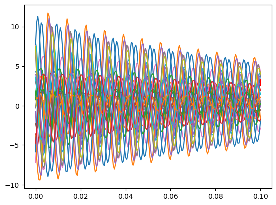
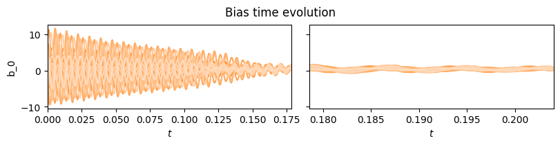
filter_ens.visualize_history(truth=truth)

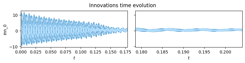
v. Plot results¶

Exercise¶

How does the solution change as we vary the bias regularization factor, $\gamma$ ? What happens if $\gamma=0$? And if $\gamma=25$?

# Check the training data and results training_data = np.load(f'{training_data_filename}', allow_pickle=True) data = training_data.get('data') data.shape b_prediction = filter_ens.bias.get_bias_hist(mean=True) plt.figure(figsize=(12, 5)) time = truth.t_true[:len(data[1])] - truth.t_true[0] # plt.plot(time, truth.b_true[:len(data[1]), 0], label='True bias', c='k', lw=2) zeros = np.zeros_like(data[...,0]) + np.mean(data[...,0], axis=1, keepdims=True) plt.bar(np.arange(data.shape[0]), sorted(np.mean(data[...,0], axis=1))) # plt.plot(time, zeros.T, label='Training data', alpha=0.5) # plt.plot(filter_ens.bias.hist_t-filter_ens.bias.hist_t[0], b_prediction[:, 0], label='Predicted bias', c='r', lw=2 # log lims # plt.gca().set_yscale('log') # plt.xlim(time[0], time[500])

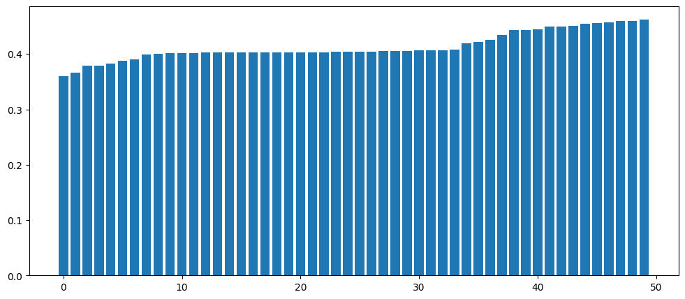
<BarContainer object of 50 artists>