Skip to content

Echo State Network model

ESN_model combines a discrete-time forecast model with the reservoir core provided by echostatenetwork. The main configuration parameters control the reservoir size, spectral radius, input scaling, and washout.

romda.models.data_driven.rnns.esn.ESN_model(dt, **kwargs)

Bases: EchoStateNetwork, Model

Echo state network as a data-driven forecast model.

Wraps the EchoStateNetwork reservoir with the Model interface (state history, discrete integrator, observation operator), so a trained ESN can be used as the forecast model of an Ensemble — or as the forecaster inside ESN_bias. The model state is \([\mathbf{u}; \mathbf{r}]\): the physical outputs and the reservoir state. Training data is mandatory at construction (the network trains itself unless a cached configuration is found).

Parameters:

Name Type Description Default
dt float

Output time step (the internal ESN step is dt * upsample).

required
**kwargs

Supported keys include:

  • data : np.ndarray, training data, shape \((L, N_t, N_\mathrm{dim})\) (\(L\) segments/experiments, \(N_t\) time steps spanning train + validation + test, \(N_\mathrm{dim}\) state dimensions). Required unless y0 is given (with pre-trained matrices, e.g. Wout).
  • y0 : np.ndarray, initial state, used only if data is not given.
  • plot_training : bool, whether to plot the training data and convergence. Default True.
  • ESN hyperparameters (N_units, N_wash, rho_range, ...) and Model options.
{}
Source code in src/models/data_driven/rnns/esn.py
 86
 87
 88
 89
 90
 91
 92
 93
 94
 95
 96
 97
 98
 99
100
101
102
103
104
105
106
107
108
109
110
111
112
113
114
115
116
117
118
119
120
121
122
123
124
125
126
127
128
129
130
131
132
133
134
135
136
137
138
139
140
141
142
143
144
145
146
147
148
149
150
151
152
153
154
155
156
157
158
159
160
161
162
163
164
165
166
167
168
169
170
171
172
def __init__(self,
             dt,
             **kwargs):
    # See the class docstring for the meaning of dt and **kwargs.
    data = kwargs.pop('data', None)
    y0 = kwargs.pop('y0', None)
    plot_training = kwargs.pop('plot_training', True)

    # =================== STEP 0: ESTIMABLE INPUT PARAMETERS ======================
    # A parametric ESN is conditioned on a physical parameter vector that is
    # normally *given* at forecast time (`EchoStateNetwork.input_parameters`).
    # Naming the entries in `param_names` mirrors each one as a `Model` parameter:
    # it can be listed in `est_alpha`, joins the augmented state alongside the
    # reservoir (and the `Wout` singular values), and is read back per member
    # before every forecast (see `time_step`). `param_values` are the nominal
    # values (the ensemble mean at initialization). Avoid the names of the ESN's
    # own hyperparameters (`rho`/`sigma_in`/`tikh`).
    self.param_names = tuple(kwargs.pop('param_names', ()))
    param_labels = kwargs.pop('param_labels', None)
    values = np.atleast_1d(np.asarray(
        kwargs.pop('param_values', np.zeros(len(self.param_names))), dtype=float))
    # kept as attributes so the config store can save/rebuild a parametric ESN
    self.param_values = tuple(float(v) for v in values)
    self.param_labels = tuple(param_labels) if param_labels else None
    for name, val in zip(self.param_names, values):
        setattr(self, name, float(val))
    # `Model.__init__` builds alpha0 from `params`, so register them before it runs
    self.params = list(self.params) + list(self.param_names)

    # =================== STEP 1: EchoStateNetwork INITIALIZATION ======================

    [setattr(self, key, kwargs.pop(key)) for key in list(kwargs.keys()) if key in vars(ESN_model)]

    if data is not None:
        assert isinstance(data, np.ndarray), f"Expected data to be a numpy array, got {type(data)}"
        data = self._process_initialization_data(data, dt, kwargs) # type: np.ndarray # with shape (L, Nt, Ndim)
        y0 = data[0, 0]
    elif y0 is None:
        raise ValueError('Either training data or initial state y0 must be provided to initialize the ESN_model.')

    initial_dict = {key: kwargs.pop(key) for key in list(kwargs.keys()) if key in vars(EchoStateNetwork)}
    EchoStateNetwork.__init__(self,
                            y=y0,
                            dt=dt,
                            **initial_dict)


    # =================== STEP 2: EchoStateNetwork TRAINING ======================
    # Train the network if not already trained
    if not self.trained:
        print('Training ESN model...')
        if plot_training:
            self.plot_training_data(case=self, train_data=data, dt=dt)

        self.train(train_data=data, plot_training=plot_training, **kwargs)

        # save validation data for initialization
        Y_wtv = self._split_and_format_data(data)[1]
        self.validation_data = Y_wtv[-(self.N_wash + self.N_val):]


    # ================== STEP 3: DEFINE INITIAL STATE & PARAMS ======================
    # `Model.Nq = 1` is a class attribute, so `hasattr` is always True -- check the
    # instance dict instead, otherwise every ESN_model silently ends up with Nq=1
    # (POD_ESN sets its own Nq as an instance attribute before calling this).
    if 'Nq' not in vars(self):
        self.Nq = len(self.observed_idx)  # Number of observed dimensions (for the physical state)

    psi0 = self.initialize_from_val_data()  # shape (Ndim + N_units + Na, m)

    # Initialise SVD Wout terms if required
    if self.Wout_svd:
        [self.Wout_U, self.Wout_Sigma0, self.Wout_Vh] = sla.svd(self.Wout, full_matrices=False)
        self.Wout_Sigma = self.Wout_Sigma0

    # =================== STEP 4: Model INITIALIZATION ======================
    Model.__init__(self,
                   dt=dt,
                   psi0=psi0,
                   integrator_class=DiscreteIntegrator,
                   **kwargs)

    if self.param_names:
        # `Model.alpha_labels` defaults to a label->name mapping, so plotting an
        # estimated parameter by name raises KeyError until real labels are set.
        self.alpha_labels = dict(zip(self.param_names,
                                     param_labels or [f'${n}$' for n in self.param_names]))

t_transient property

float: Total time spanning training + validation + test, t_train + t_val + t_test.

dt_step property

float: Integrator time step, dt_ESN (the ESN advances in closed loop at its own upsampled time step, not dt).

t_CR property

float: Characteristic response time used by the base Model, aliased to t_val.

Wout_U property writable

np.ndarray: Left singular vectors of Wout (from scipy.linalg.svd(Wout, full_matrices=False)), shape Wout.shape i.e. (N_units + 1, N_dim). Only used/set when Wout_svd is True.

Wout_Vh property writable

np.ndarray: Right singular vectors of Wout (transposed), shape (N_dim, N_dim). Only used/set when Wout_svd is True.

Wout_Sigma property writable

np.ndarray: Ensemble of diagonal singular-value matrices used to reconstruct Wout as \(\mathbf{W}_\mathrm{out} \approx \mathbf{U}\,\boldsymbol{\Sigma}\,\mathbf{V}^\mathrm{h}\) (see reservoir_to_physical), shape (m, N_dim, N_dim). If Wout_svd, recomputed from the current svd_i ensemble parameters on every access (via alpha_to_Sigma); otherwise held fixed at whatever was last set.

alpha_to_Sigma property

np.ndarray: Per-ensemble-member diagonal singular-value matrices built from the current svd_i parameter estimates (get_alpha_matrix), falling back to the corresponding Wout_Sigma0 singular value for any svd_i not in est_alpha. Shape (m, N_dim, N_dim).

get_alpha_matrix property

np.ndarray: Current ensemble parameter estimates (est_alpha), shape (len(est_alpha), m), read from get_alpha.

Wout_Sigma0 property writable

np.ndarray: Reference (initial) singular values of Wout, shape (N_dim,), as computed by scipy.linalg.svd when Wout_svd is enabled.

N_ens property

int: Ensemble size, read from ensemble['m'] if an ensemble configuration is set, otherwise the trailing dimension of current_state.

state_labels property

list of str: LaTeX labels for the state vector, \(u_1, \dots, u_{N_\mathrm{dim}}\) (physical outputs) followed by \(r_1, \dots, r_{N_\mathrm{units}}\) (reservoir units).

obs_labels property

list of str: LaTeX labels for the observed physical outputs (observed_idx).

reservoir_state property

np.ndarray: Reservoir-state block of current_state, shape (N_units, m).

modify_settings(**kwargs)

Update existing attributes in place, switching to the SVD parametrization of Wout (see Wout_svd) if 'Wout' is requested as an ensemble parameter to estimate (est_alpha).

Parameters:

Name Type Description Default
**kwargs

Attribute name/value pairs to set; each name must already exist on the instance.

{}

Returns:

Type Description
None

Updates attributes (and, if applicable, est_alpha/alpha_labels/ alpha_lims/M) in place.

Raises:

Type Description
ValueError

If a key in kwargs is not an existing attribute.

Source code in src/models/data_driven/rnns/esn.py
220
221
222
223
224
225
226
227
228
229
230
231
232
233
234
235
236
237
238
239
240
241
242
243
244
245
246
247
248
249
250
251
252
253
254
255
256
257
258
259
260
261
262
263
264
265
266
267
268
269
def modify_settings(self, **kwargs):
    """Update existing attributes in place, switching to the SVD parametrization
    of `Wout` (see `Wout_svd`) if ``'Wout'`` is requested as an ensemble parameter
    to estimate (`est_alpha`).

    Parameters
    ----------
    **kwargs
        Attribute name/value pairs to set; each name must already exist on the
        instance.

    Returns
    -------
    None
        Updates attributes (and, if applicable, `est_alpha`/`alpha_labels`/
        `alpha_lims`/`M`) in place.

    Raises
    ------
    ValueError
        If a key in `kwargs` is not an existing attribute.
    """
    for key, val in kwargs.items():
        if hasattr(self, key):
            setattr(self, key, val)
        else:
            raise ValueError(f'Key {key} not in ESN_model class')


    if self.ensemble_cfg is not None:
        # If Wout is being estimated, we need to update the est_alpha list to include the SVD components
        # and remove Wout. We do not directly estimate Wout, but rather its singular values.
        if 'Wout' in self.est_alpha:
            self.est_alpha = [a for a in self.est_alpha if a != 'Wout'] + \
                             [f'svd_{qi}' for qi in range(self.N_dim)]

        # The switch must key on the svd names, not on 'Wout': callers that build
        # the initial ensemble themselves (esn_ensemble) pass est_alpha already
        # expanded, and without Wout_svd the read-out keeps using the fixed Wout —
        # the estimated singular values never act on the forecast.
        svd_keys = [a for a in self.est_alpha if a.startswith('svd_')]
        if svd_keys:
            if not self.Wout_svd:
                self.Wout_svd = True
                [self.Wout_U, self.Wout_Sigma0, self.Wout_Vh] = sla.svd(self.Wout, full_matrices=False)
                self.Wout_Sigma = self.Wout_Sigma0
            # the setters merge, so labels/lims of other estimated parameters survive
            self.alpha_labels = {key: f'$\\sigma_{{{key.split("_")[1]}}}$' for key in svd_keys}
            self.alpha_lims = {key: (None, None) for key in svd_keys}
    self.M = None

init_ensemble(m=10, est_alpha=[], std_alpha=0.001, distribution_alpha='uniform', regimes=None, seed=0, measured=None, ensemble_psi0=None, **kwargs)

ESN override of Model.init_ensemble: members start from reservoir states visited during training (initialize_from_val_data) — the generic transient + multiplicative std_phi path pushes r outside the tanh range and the closed loop blows up.

regimes ((N_param, L), parametric ESN): washes each member out on one training segment and starts it from that segment's parameters, keeping state and parameter consistent — paired independently, members leave the learned attractor and diverge. 'Wout' in est_alpha estimates the read-out singular values (one svd_i per output dimension); measured restricts the observation operator to those state components.

Parameter perturbations draw from this instance's rng; an estimator builds the ensemble on its own copy (EnsembleEstimator copies parent_model first), so repeated builds from one parent network draw identical perturbations — the parent's rng is deliberately untouched.

Source code in src/models/data_driven/rnns/esn.py
438
439
440
441
442
443
444
445
446
447
448
449
450
451
452
453
454
455
456
457
458
459
460
461
462
463
464
465
466
467
468
469
470
471
472
473
474
475
476
477
478
479
480
481
482
483
484
485
486
487
488
489
490
491
492
493
494
495
496
497
498
499
500
501
502
503
504
505
506
507
508
509
def init_ensemble(self, m=10, est_alpha=[], std_alpha=0.001,
                  distribution_alpha='uniform', regimes=None, seed=0,
                  measured=None, ensemble_psi0=None, **kwargs):
    """ESN override of `Model.init_ensemble`: members start from reservoir states
    visited during training (`initialize_from_val_data`) — the generic transient +
    multiplicative `std_phi` path pushes `r` outside the tanh range and the closed
    loop blows up.

    `regimes` (`(N_param, L)`, parametric ESN): washes each member out on one
    training segment *and* starts it from that segment's parameters, keeping state
    and parameter consistent — paired independently, members leave the learned
    attractor and diverge. ``'Wout'`` in `est_alpha` estimates the read-out
    singular values (one ``svd_i`` per output dimension); `measured` restricts
    the observation operator to those state components.

    Parameter perturbations draw from *this* instance's `rng`; an estimator
    builds the ensemble on its own copy (`EnsembleEstimator` copies
    `parent_model` first), so repeated builds from one parent network draw
    identical perturbations — the parent's `rng` is deliberately untouched."""
    if ensemble_psi0 is None:
        nominal = {}
        if isinstance(std_alpha, dict) and 'Wout' in std_alpha:
            std_alpha = dict(std_alpha)
            std_alpha.update({f'svd_{qi}': std_alpha.pop('Wout')
                              for qi in range(self.N_dim)})
        if isinstance(std_alpha, dict) and not est_alpha:
            # base-class convention: an empty est_alpha with a dict std_alpha
            # estimates every parameter in the dict; an explicit est_alpha is
            # honored (the dict may carry spreads for more parameters)
            est_alpha = sorted(std_alpha)
        if 'Wout' in est_alpha:
            svd_names = [f'svd_{qi}' for qi in range(self.N_dim)]
            est_alpha = [a for a in est_alpha if a != 'Wout'] + svd_names
            nominal = dict(zip(svd_names, sla.svd(self.Wout, full_matrices=False)[1]))

        if regimes is None:
            phi, alpha = self.initialize_from_val_data(N_ens=m), {}
        else:
            phi, values = self._regime_matched_init(m, np.atleast_2d(regimes), seed=seed)
            alpha = dict(zip(self.param_names, values))

        other = [a for a in est_alpha if a not in alpha]
        if other:
            means = [nominal.get(a, getattr(self, a, None)) for a in other]
            assert not any(v is None for v in means), \
                f'init_ensemble: no nominal value to seed the ensemble for {other}'
            sub_std = ({a: std_alpha[a] for a in other}
                       if isinstance(std_alpha, dict) else std_alpha)
            alpha.update(zip(other, mean_vector_to_ensemble(
                self.rng, np.array(means, dtype=float), sub_std, m,
                method=distribution_alpha)))

        ensemble_psi0 = phi if not est_alpha else np.concatenate(
            [phi, np.stack([alpha[name] for name in est_alpha])], axis=0)

    out = super().init_ensemble(m=m, est_alpha=est_alpha, std_alpha=std_alpha,
                                distribution_alpha=distribution_alpha,
                                ensemble_psi0=ensemble_psi0, **kwargs)

    if measured is not None:
        if np.isscalar(measured):   # int count or digit string: resolve to indices
            from romda.observations import measured_idx
            idx = measured_idx(measured, self.N_dim)
        else:
            idx = [int(k) for k in measured]
        if idx != list(self.observed_idx):
            # Rows of `M` for the measured components only. Written to the private
            # attribute: the public setter requires exactly Nq rows, and a
            # restricted operator deliberately has fewer.
            obs = list(self.observed_idx)
            self._M = self.M[[obs.index(k) for k in idx]]
    return out

initialize_from_val_data(N_ens=1, seed=0)

Initialize the ESN state (physical output and reservoir) from an open-loop washout over a random time window of validation_data, so a fresh ensemble starts from an on-attractor reservoir state rather than zeros.

Parameters:

Name Type Description Default
N_ens int

Number of ensemble members (random washout windows) to draw. Default 1.

1
seed int

Random seed for selecting the washout windows. Overridden by self.seed if set.

0

Returns:

Type Description
ndarray

Initial full state (built via build_psi), shape (N_dim + N_units [+ Na], N_ens).

Raises:

Type Description
AssertionError

If validation_data has not been set (i.e. before training).

Source code in src/models/data_driven/rnns/esn.py
535
536
537
538
539
540
541
542
543
544
545
546
547
548
549
550
551
552
553
554
555
556
557
558
559
560
561
562
563
564
565
566
567
568
569
570
571
572
573
574
575
576
577
578
579
580
581
582
583
584
585
586
587
588
589
590
591
592
593
594
595
596
597
598
599
600
601
602
603
604
605
606
def initialize_from_val_data(self, N_ens=1, seed=0):
    """Initialize the ESN state (physical output and reservoir) from an
    open-loop washout over a random time window of `validation_data`, so a fresh
    ensemble starts from an on-attractor reservoir state rather than zeros.

    Parameters
    ----------
    N_ens : int
        Number of ensemble members (random washout windows) to draw. Default 1.
    seed : int
        Random seed for selecting the washout windows. Overridden by `self.seed`
        if set.

    Returns
    -------
    np.ndarray
        Initial full state (built via `build_psi`), shape
        ``(N_dim + N_units [+ Na], N_ens)``.

    Raises
    ------
    AssertionError
        If `validation_data` has not been set (i.e. before training).
    """
    assert self.validation_data is not None

    data = self.validation_data.copy()

    if hasattr(self, 'seed'):
        seed = self.seed
    rng0 = np.random.default_rng(seed)


    # initialise state with a random sample from test data
    u_init, r_init = np.empty((self.N_dim, N_ens)), np.empty((self.N_units, N_ens))

    # Random time windows and dimension
    if data.shape[0] == 1:
        dim_ids = [0] * N_ens
    else:
        # Choose a random dimension from the data
        replace = N_ens >= data.shape[0]
        dim_ids = rng0.choice(data.shape[0], size=N_ens, replace=replace)

    # Choose random time indices from the data (with replacement when there are
    # fewer washout windows than members, e.g. a short validation record)
    n_windows = data.shape[1] - self.N_wash
    t_ids = rng0.choice(n_windows, size=N_ens, replace=N_ens >= n_windows)

    # validation_data is indexed by segment (dim_i matches a column of
    # input_parameters); condition the washout of each segment on its own
    # parameter vector, then restore the full (N_param, L) array afterwards.
    original_input_parameters = self.input_parameters

    for ii, ti, dim_i in zip(range(N_ens), t_ids, dim_ids):
        u_wash = data[dim_i, ti:ti+self.N_wash]
        r_open = np.zeros((self.N_units, 1))
        u_open = np.zeros((self.N_dim, 1))
        if original_input_parameters is not None:
            self.input_parameters = original_input_parameters[:, dim_i]
        # Open-loop reservoir
        for u_in in u_wash:
            u_open, r_open = self._single_step(u_in, r_open)

        #store final state into the initialization arrays
        u_init[:, ii] = u_open.squeeze()
        r_init[:, ii] = r_open.squeeze()

    self.input_parameters = original_input_parameters

    # Set physical and reservoir states as ensembles
    return self.build_psi(u=u_init, r=r_init)

closed_loop(data, n_steps, input_parameters=None)

Open-loop washout on data[:N_wash] (sampled at dt_ESN), then a closed-loop forecast; returns (prediction, target), both (n_steps, N_dim).

The ESN maps u_t to u_{t+1}, so the last washout step already predicts data[N_wash] — an off-by-one here costs a full dt_ESN of drift.

Source code in src/models/data_driven/rnns/esn.py
609
610
611
612
613
614
615
616
617
618
619
620
621
622
623
624
625
626
627
628
629
630
631
632
633
634
def closed_loop(self, data, n_steps, input_parameters=None):
    """Open-loop washout on `data[:N_wash]` (sampled at `dt_ESN`), then a closed-loop
    forecast; returns ``(prediction, target)``, both `(n_steps, N_dim)`.

    The ESN maps `u_t` to `u_{t+1}`, so the *last* washout step already predicts
    `data[N_wash]` — an off-by-one here costs a full `dt_ESN` of drift."""
    original = self.input_parameters
    if input_parameters is not None:
        self.input_parameters = np.asarray(input_parameters, dtype=float).reshape(-1, 1)

    try:
        r = np.zeros((self.N_units, 1))
        u = np.zeros((self.N_dim, 1))
        for u_in in data[:self.N_wash]:
            u, r = self.step(self.outputs_to_inputs(np.asarray(u_in)[:, np.newaxis]), r)

        pred = np.empty((n_steps, self.N_dim))
        pred[0] = u[:, 0]
        for i in range(1, n_steps):
            u, r = self._single_step(u, r)
            pred[i] = u[:, 0]
    finally:
        # the training-time (N_param, L) array must survive a single-regime forecast
        self.input_parameters = original

    return pred, np.asarray(data[self.N_wash:self.N_wash + n_steps])

reset_ESN(data, u0=None, plot_training=False, **kwargs)

Reinitialize and retrain the underlying EchoStateNetwork from scratch on new data, then reset the Model state/history around the freshly trained network.

Parameters:

Name Type Description Default
data ndarray

New training data, shape (L, Nt, N_dim); forwarded to train.

required
u0 ndarray

Initial physical state for the new EchoStateNetwork. Defaults to the physical state corresponding to the current reservoir_state.

None
plot_training bool

Whether to plot the (re-)training process. Default False.

False
**kwargs

ESN hyperparameters (forwarded to EchoStateNetwork.__init__), training options (forwarded to train) and Model reset options (forwarded to reset_model).

{}

Returns:

Type Description
None

Reinitializes self in place.

Source code in src/models/data_driven/rnns/esn.py
637
638
639
640
641
642
643
644
645
646
647
648
649
650
651
652
653
654
655
656
657
658
659
660
661
662
663
664
665
666
667
668
669
670
671
672
673
674
675
676
677
678
679
def reset_ESN(self, data, u0=None, plot_training=False, **kwargs):
    """Reinitialize and retrain the underlying `EchoStateNetwork` from scratch
    on new `data`, then reset the `Model` state/history around the freshly
    trained network.

    Parameters
    ----------
    data : np.ndarray
        New training data, shape ``(L, Nt, N_dim)``; forwarded to `train`.
    u0 : np.ndarray, optional
        Initial physical state for the new `EchoStateNetwork`. Defaults to the
        physical state corresponding to the current `reservoir_state`.
    plot_training : bool
        Whether to plot the (re-)training process. Default False.
    **kwargs
        ESN hyperparameters (forwarded to `EchoStateNetwork.__init__`), training
        options (forwarded to `train`) and `Model` reset options (forwarded to
        `reset_model`).

    Returns
    -------
    None
        Reinitializes `self` in place.
    """
    if u0 is None:
        u0 = self.reservoir_to_physical(self.reservoir_state)

    EchoStateNetwork.__init__(self,
                              y=u0,
                              dt=self.dt,
                              figs_folder=self.results_folder,
                              **kwargs)
    # Train the network
    possible_args = inspect.getfullargspec(self.train)[0]
    train_args = {key: val for key, val in kwargs.items() if key in possible_args}

    # Train network
    self.train(train_data=data, plot_training=plot_training, **train_args)


    # Reset model class
    kwargs['psi0'] = self.build_psi()
    self.reset_model(**kwargs)

get_observables(Nt=1, **kwargs)

Observables are the observed physical outputs, which need not be the leading rows of psi (the base Model assumes psi[:Nq]).

Parameters:

Name Type Description Default
Nt int

Number of trailing history steps to return. Default 1.

1
**kwargs

Unused; accepted for interface compatibility.

{}

Returns:

Type Description
ndarray

Observed outputs, shape (Nq, m) if Nt == 1 else (Nt, Nq, m).

Source code in src/models/data_driven/rnns/esn.py
698
699
700
701
702
703
704
705
706
707
708
709
710
711
712
713
714
715
716
def get_observables(self, Nt=1, **kwargs):
    """Observables are the *observed* physical outputs, which need not be the
    leading rows of psi (the base Model assumes `psi[:Nq]`).

    Parameters
    ----------
    Nt : int
        Number of trailing history steps to return. Default 1.
    **kwargs
        Unused; accepted for interface compatibility.

    Returns
    -------
    np.ndarray
        Observed outputs, shape ``(Nq, m)`` if ``Nt == 1`` else ``(Nt, Nq, m)``.
    """
    if Nt == 1:
        return self.hist[-1, self.observed_idx, :]
    return self.hist[-Nt:, self.observed_idx, :]

reservoir_to_physical(r)

Convert reservoir states to physical outputs via Wout (overrides EchoStateNetwork.reservoir_to_physical to also support the SVD parametrization of Wout, see Wout_svd).

When Wout_svd is False: \(\mathbf{u} = \mathbf{W}_\mathrm{out}^\mathrm{T}[\mathbf{r}; b_\mathrm{out}]\), as in the base class. When True, \(\mathbf{W}_\mathrm{out}\) is reconstructed (per ensemble member, if r has m members) from \(\mathbf{U}\,\boldsymbol{\Sigma}\,\mathbf{V}^\mathrm{h}\) (Wout_U, Wout_Sigma, Wout_Vh) before the same read-out is applied; if r does not have exactly m members (e.g. a single averaged state), Wout_Sigma is averaged over the ensemble first.

Parameters:

Name Type Description Default
r ndarray

Reservoir state, shape (N_units, N_ens).

required

Returns:

Type Description
ndarray

Physical output, shape (N_dim, N_ens).

Source code in src/models/data_driven/rnns/esn.py
726
727
728
729
730
731
732
733
734
735
736
737
738
739
740
741
742
743
744
745
746
747
748
749
750
751
752
753
754
755
756
757
758
759
760
761
762
763
764
def reservoir_to_physical(self, r):
    r"""Convert reservoir states to physical outputs via `Wout` (overrides
    `EchoStateNetwork.reservoir_to_physical` to also support the SVD
    parametrization of `Wout`, see `Wout_svd`).

    When `Wout_svd` is False: $\mathbf{u} = \mathbf{W}_\mathrm{out}^\mathrm{T}[\mathbf{r}; b_\mathrm{out}]$,
    as in the base class. When True, $\mathbf{W}_\mathrm{out}$ is reconstructed
    (per ensemble member, if `r` has `m` members) from
    $\mathbf{U}\,\boldsymbol{\Sigma}\,\mathbf{V}^\mathrm{h}$ (`Wout_U`, `Wout_Sigma`,
    `Wout_Vh`) before the same read-out is applied; if `r` does not have exactly
    `m` members (e.g. a single averaged state), `Wout_Sigma` is averaged over the
    ensemble first.

    Parameters
    ----------
    r : np.ndarray
        Reservoir state, shape ``(N_units, N_ens)``.

    Returns
    -------
    np.ndarray
        Physical output, shape ``(N_dim, N_ens)``.
    """
    bias_out = self.bias_out * np.ones((1, r.shape[-1]))
    r_aug = np.concatenate((r, bias_out), axis=0)

    if not self.Wout_svd:
        return np.dot(r_aug.T, self.Wout).T
    else:

        if r.shape[-1] == self.m:
            Wout = np.einsum('ij,kjl,lm->imk', self.Wout_U, self.Wout_Sigma, self.Wout_Vh)
            return np.einsum('ij,ikj->kj', r_aug, Wout)
        else:
            # average the alpha values
            print('Averaging Wout_Sigma for reservoir_to_physical')
            Wout_Sigma_avg = np.mean(self.Wout_Sigma, axis=0)
            Wout = np.dot(self.Wout_U, np.dot(Wout_Sigma_avg, self.Wout_Vh))
            return np.dot(r_aug.T, Wout).T

time_step(Nt=10, averaged=False)

Advance the ESN in closed loop.

Parameters:

Name Type Description Default
Nt int

Number of forecast steps (in physical time steps, not dt_ESN).

10
averaged bool

If True, the ensemble is forecast as its mean plus frozen deviations; otherwise each member is forecast individually.

False

Returns:

Type Description
tuple

(psi, t) — forecasted state of shape (Nt+1, N, m) and the corresponding times.

Source code in src/models/data_driven/rnns/esn.py
775
776
777
778
779
780
781
782
783
784
785
786
787
788
789
790
791
792
793
794
795
796
797
798
799
800
801
802
803
804
805
806
807
808
809
810
811
812
813
814
815
816
817
818
819
820
821
822
823
824
825
826
827
828
829
830
831
832
833
def time_step(self, Nt=10, averaged=False):
    """Advance the ESN in closed loop.

    Parameters
    ----------
    Nt : int
        Number of forecast steps (in physical time steps, not ``dt_ESN``).
    averaged : bool
        If True, the ensemble is forecast as its mean plus frozen deviations;
        otherwise each member is forecast individually.

    Returns
    -------
    tuple
        ``(psi, t)`` — forecasted state of shape ``(Nt+1, N, m)`` and the
        corresponding times.
    """

    assert self.trained, 'ESN model not trained'

    if self.param_names:
        # Condition each member's forecast on its own current parameter value.
        # `get_alpha` returns one dict per member: the estimated value when the
        # parameter is in `est_alpha`, otherwise the nominal `alpha0` one (change
        # it in place with ``esn.alpha0[name] = ...`` to forecast at a fixed
        # parameter). Either way the `(N_param, m)` array replaces the
        # `(N_param, L)` one left over from training.
        alpha = self.get_alpha()
        self.input_parameters = np.array([[a[name] for a in alpha]
                                          for name in self.param_names])

    # 1. get initial condition


    t = np.round(self.current_time + np.arange(0, Nt + 1) * self.dt_ESN, self.precision_t)
    psi0 = self.current_state
    u, r_out = np.empty((Nt + 1, self.N_dim, self.m)), np.empty((Nt + 1, self.N_units, self.m))
    u[0], r_out[0] = self.unbuild_psi(psi0)

    if averaged:
        # Mean state
        u_m, r_m = (np.mean(yy[0], axis=-1, keepdims=True) for yy in [u, r_out])
        u_dev, r_dev = u[0] - u_m[0], r_out[0] - r_m[0]


        for i in range(Nt):
            u_m, r_m = self._single_step(u_m, r_m)
            u[i+1] = u_m + u_dev
            r_out[i+1] = r_m + r_dev

    else:

        for i in range(Nt):
            u[i+1], r_out[i+1] = self._single_step(u[i], r_out[i])


    psi = self.build_psi(u=u, r=r_out)

    return psi, t

build_psi(u=None, r=None)

Assemble the full model state from physical output u and reservoir state r: concatenate([u, r, alpha]) along the state axis, keeping only u or only r if update_state/update_reservoir is False, and appending the ensemble parameter block (get_alpha_matrix) if Na > 0.

Parameters:

Name Type Description Default
u ndarray

Physical output, shape (N_dim, m) or (Nt, N_dim, m). Defaults to reservoir_to_physical(r).

None
r ndarray

Reservoir state, shape (N_units, m) or (Nt, N_units, m). Defaults to reservoir_state.

None

Returns:

Type Description
ndarray

Full state psi, shape (N [+ Na], m) or (Nt, N [+ Na], m).

Raises:

Type Description
ValueError

If u and r have incompatible number of dimensions, or (for 3D inputs) a mismatched number of time steps.

Source code in src/models/data_driven/rnns/esn.py
841
842
843
844
845
846
847
848
849
850
851
852
853
854
855
856
857
858
859
860
861
862
863
864
865
866
867
868
869
870
871
872
873
874
875
876
877
878
879
880
881
882
883
884
885
886
887
888
889
890
891
892
893
894
895
896
def build_psi(self, u=None, r=None):
    """Assemble the full model state from physical output `u` and reservoir
    state `r`: ``concatenate([u, r, alpha])`` along the state axis, keeping only
    `u` or only `r` if `update_state`/`update_reservoir` is False, and appending
    the ensemble parameter block (`get_alpha_matrix`) if `Na > 0`.

    Parameters
    ----------
    u : np.ndarray, optional
        Physical output, shape ``(N_dim, m)`` or ``(Nt, N_dim, m)``. Defaults to
        `reservoir_to_physical(r)`.
    r : np.ndarray, optional
        Reservoir state, shape ``(N_units, m)`` or ``(Nt, N_units, m)``. Defaults
        to `reservoir_state`.

    Returns
    -------
    np.ndarray
        Full state ``psi``, shape ``(N [+ Na], m)`` or ``(Nt, N [+ Na], m)``.

    Raises
    ------
    ValueError
        If `u` and `r` have incompatible number of dimensions, or (for 3D
        inputs) a mismatched number of time steps.
    """
    if r is None:
        r = self.reservoir_state
    if u is None:
        u = self.reservoir_to_physical(r)


    if u.ndim == 2 and r.ndim == 2:
        ax_dim = 0
    elif u.ndim == 3 and r.ndim == 3:
        ax_dim = 1
        if u.shape[0] != r.shape[0]:
            raise ValueError(f'Incompatible time steps for u ({u.shape[0]}) and r ({r.shape[0]})')
    else:
        raise ValueError(f'Incompatible dimensions for u ({u.ndim}) and r ({r.ndim})')

    if self.update_state and self.update_reservoir:
        phi = np.concatenate((u, r), axis=ax_dim)
    elif self.update_state:
        phi = u
    else:
        phi = r


    if self.Na > 0:
        alph = self.get_alpha_matrix
        if u.ndim == 3:
            alph = np.tile(alph, reps=(u.shape[0], 1, 1)) # repeat for all time steps (alpha is constant in time)
        return np.concatenate((phi, alph), axis=ax_dim)
    else:
        return phi

unbuild_psi(psi=None)

Inverse of build_psi: split a full state vector into its physical (u) and reservoir (r) blocks, assuming they occupy the leading N_dim + N_units rows of psi (as build_psi lays them out when both update_state and update_reservoir are True).

Parameters:

Name Type Description Default
psi ndarray

Full state, shape (N, m) or (Nt, N, m). Defaults to current_state.

None

Returns:

Name Type Description
u ndarray

Physical state, shape (N_dim, m) (or (Nt, N_dim, m)).

r ndarray

Reservoir state, shape (N_units, m) (or (Nt, N_units, m)).

Raises:

Type Description
AssertionError

If psi has fewer than N_units + 1 rows.

Source code in src/models/data_driven/rnns/esn.py
899
900
901
902
903
904
905
906
907
908
909
910
911
912
913
914
915
916
917
918
919
920
921
922
923
924
925
926
927
928
929
930
931
932
933
934
935
936
937
938
939
def unbuild_psi(self, psi=None):
    """Inverse of `build_psi`: split a full state vector into its physical
    (`u`) and reservoir (`r`) blocks, assuming they occupy the leading
    ``N_dim + N_units`` rows of `psi` (as `build_psi` lays them out when both
    `update_state` and `update_reservoir` are True).

    Parameters
    ----------
    psi : np.ndarray, optional
        Full state, shape ``(N, m)`` or ``(Nt, N, m)``. Defaults to
        `current_state`.

    Returns
    -------
    u : np.ndarray
        Physical state, shape ``(N_dim, m)`` (or ``(Nt, N_dim, m)``).
    r : np.ndarray
        Reservoir state, shape ``(N_units, m)`` (or ``(Nt, N_units, m)``).

    Raises
    ------
    AssertionError
        If `psi` has fewer than `N_units` + 1 rows.
    """
    if psi is None:
        psi = self.current_state
    if psi.ndim == 2:
        psi = np.expand_dims(psi, axis=0)
        squeeze = True
    else:
        squeeze = False

    assert psi.shape[1] > self.N_units, f"Expected psi shape (N x m) with N > {self.N_units}, got {psi.shape}"
    u = psi[:, :self.N_dim]
    r = psi[:, self.N_dim:self.N_dim+self.N_units]

    if squeeze:
        u = u.squeeze(axis=0)
        r = r.squeeze(axis=0)

    return u, r

plot_training_data(case, train_data, dt=None) staticmethod

Plot each dimension of train_data, shading the training/validation/test windows (case.t_train/t_val/t_test).

Parameters:

Name Type Description Default
case ESN_model

Instance providing t_train, t_val, t_test (and dt if not given).

required
train_data ndarray

Data to plot, shape (L, Nt, N_dim) (or 1D/2D, reshaped accordingly).

required
dt float

Time step for the x-axis. Defaults to case.dt.

None

Returns:

Type Description
None

Displays the figure with matplotlib.pyplot.show.

Source code in src/models/data_driven/rnns/esn.py
 944
 945
 946
 947
 948
 949
 950
 951
 952
 953
 954
 955
 956
 957
 958
 959
 960
 961
 962
 963
 964
 965
 966
 967
 968
 969
 970
 971
 972
 973
 974
 975
 976
 977
 978
 979
 980
 981
 982
 983
 984
 985
 986
 987
 988
 989
 990
 991
 992
 993
 994
 995
 996
 997
 998
 999
1000
@staticmethod
def plot_training_data(case, train_data, dt=None):
    """Plot each dimension of `train_data`, shading the training/validation/test
    windows (`case.t_train`/`t_val`/`t_test`).

    Parameters
    ----------
    case : ESN_model
        Instance providing `t_train`, `t_val`, `t_test` (and `dt` if not given).
    train_data : np.ndarray
        Data to plot, shape ``(L, Nt, N_dim)`` (or 1D/2D, reshaped accordingly).
    dt : float, optional
        Time step for the x-axis. Defaults to ``case.dt``.

    Returns
    -------
    None
        Displays the figure with `matplotlib.pyplot.show`.
    """
    if train_data.ndim == 1:
        train_data = train_data[np.newaxis, :, np.newaxis]
    elif train_data.ndim == 2:
        train_data = train_data[np.newaxis, :]

    L, Nt, Ndim = train_data.shape
    if dt is None:
        dt = case.dt
    t_data = np.arange(0, Nt) * dt
    nrows = min(Ndim*L, 10)


    _, axs = plt.subplots(nrows=nrows, ncols=1,
                            figsize=(8, nrows), sharex=True,
                            layout='constrained')
    if nrows * L > 1 and isinstance(axs, np.ndarray):
        axs = axs.T.flatten()
    else:
        axs = [axs]


    for l, data_l in enumerate(train_data):
        axs_dim = axs[l*Ndim:(l+1)*Ndim]

        for kk, ax in enumerate(axs_dim):

            ax.plot(t_data, data_l[:, kk], lw=1., color='k')
            ax.axvspan(0, case.t_train, facecolor='orange',
                       alpha=0.3, zorder=-100, label='Train')
            ax.axvspan(case.t_train, case.t_train + case.t_val,
                       facecolor='red', alpha=0.3, zorder=-100, label='Validation')
            ax.axvspan(case.t_train + case.t_val,
                       case.t_train + case.t_val + case.t_test, facecolor='navy',
                       alpha=0.2, zorder=-100, label='Test')

            ax.legend(ncols=1, loc='upper left', bbox_to_anchor=(1., 1.), frameon=False, title=f'L={l}, dim={kk}', fontsize='x-small', title_fontsize='small')
    axs[-1].set(xlabel='time')
    plt.show()

visualize_config()

Plot the trained read-out matrix (plot_Wout).

Returns:

Type Description
None
Source code in src/models/data_driven/rnns/esn.py
1002
1003
1004
1005
1006
1007
1008
1009
def visualize_config(self):
    """Plot the trained read-out matrix (`plot_Wout`).

    Returns
    -------
    None
    """
    self.plot_Wout()

visualize_spatiotemporal_hist(y_hist=None, t=None, averaged=False, reference_y=1.0, reference_t=1.0, **kwargs)

Plot the physical and reservoir state history as space-time heat-maps (one row per state component vs. time), either per ensemble member or as the ensemble mean and standard deviation.

Parameters:

Name Type Description Default
y_hist ndarray

State history to plot, shape (Nt, N, m). Defaults to the last t_CR of hist.

None
t ndarray

Time points for y_hist. Defaults to the corresponding hist_t slice.

None
averaged bool

If True, plot the ensemble mean and standard deviation (2 rows); otherwise plot up to 10 individual state components. Default False.

False
reference_y float

Value to normalize y_hist by. Default 1.0 (no normalization).

1.0
reference_t float

Reference time used to normalize/label the time axis (see romda.utils.normalized_time). Default 1.0.

1.0
**kwargs

nrows : int, optional, number of state-component rows to plot when not averaged (default min(10, m)).

{}

Returns:

Type Description
None

Displays the figure(s) in place.

Source code in src/models/data_driven/rnns/esn.py
1062
1063
1064
1065
1066
1067
1068
1069
1070
1071
1072
1073
1074
1075
1076
1077
1078
1079
1080
1081
1082
1083
1084
1085
1086
1087
1088
1089
1090
1091
1092
1093
1094
1095
1096
1097
1098
1099
1100
1101
1102
1103
1104
1105
1106
1107
1108
1109
1110
1111
1112
1113
1114
1115
1116
1117
1118
1119
1120
1121
1122
1123
1124
1125
1126
1127
1128
1129
1130
1131
1132
1133
1134
1135
1136
1137
1138
1139
1140
1141
1142
1143
1144
1145
1146
1147
1148
1149
1150
1151
1152
1153
1154
1155
1156
1157
1158
1159
1160
1161
1162
1163
1164
1165
1166
1167
1168
1169
1170
1171
1172
1173
1174
1175
1176
1177
1178
1179
1180
1181
1182
def visualize_spatiotemporal_hist(self, y_hist=None, t=None, averaged=False,
                                  reference_y=1.0, reference_t: float = 1.0, **kwargs):
    """Plot the physical and reservoir state history as space-time heat-maps
    (one row per state component vs. time), either per ensemble member or as
    the ensemble mean and standard deviation.

    Parameters
    ----------
    y_hist : np.ndarray, optional
        State history to plot, shape ``(Nt, N, m)``. Defaults to the last
        `t_CR` of `hist`.
    t : np.ndarray, optional
        Time points for `y_hist`. Defaults to the corresponding `hist_t` slice.
    averaged : bool
        If True, plot the ensemble mean and standard deviation (2 rows);
        otherwise plot up to 10 individual state components. Default False.
    reference_y : float
        Value to normalize `y_hist` by. Default 1.0 (no normalization).
    reference_t : float
        Reference time used to normalize/label the time axis (see
        `romda.utils.normalized_time`). Default 1.0.
    **kwargs
        ``nrows`` : int, optional, number of state-component rows to plot when
        not `averaged` (default ``min(10, m)``).

    Returns
    -------
    None
        Displays the figure(s) in place.
    """
    if y_hist is None:
        n_t = int(self.t_CR // self.dt)
        y_hist = self.hist[-n_t:, :self.Nphi]

    if t is None:
        t = self.hist_t[-len(y_hist):]

    (t,), t_lbl = normalized_time(reference_t, t)
    assert t is not None
    if reference_y != 1.0:
        y_hist = y_hist / reference_y

    if y_hist.shape[1] > self.N_dim:
        y_hist_list = [y_hist[:, :self.N_dim], y_hist[:, self.N_dim:self.N_dim + self.N_units]]
        titles = ['Physical state', 'Reservoir state']
        labels = [self.state_labels[:self.N_dim], self.state_labels[self.N_dim:self.N_dim + self.N_units]]
        cmaps = ['RdBu_r', 'PRGn']
    else:
        y_hist_list = [y_hist]
        titles = ['Physical state']
        labels = [self.state_labels[:self.N_dim]]
        cmaps = ['RdBu_r']

    if not averaged:
        nrows_kw = kwargs.get('nrows', None)
        if nrows_kw is None:
            nrows = min(10, y_hist.shape[-1])
        else:
            nrows = int(nrows_kw)

        for y_hist, ttl, lbl, cmap in zip(y_hist_list, titles, labels, cmaps):
            fig, axs = plt.subplots(nrows=nrows, figsize=(10, 1.5 * nrows), sharey=True, sharex=True)
            axs_arr = np.atleast_1d(axs).ravel()
            lim = np.max(abs(y_hist))
            im = None

            for mi, ax in zip(range(nrows), axs_arr):
                im = ax.imshow(y_hist[:, :, mi].T,
                            aspect='auto', origin='lower',
                            cmap=cmap, vmin=-lim, vmax=lim,
                            extent=[t[0], t[-1], 0, y_hist.shape[1]])


            axs_arr[0].set(title=rf"ESN_model {ttl} spatiotemporal evolution. $N_\text{{units}}={self.N_units}$")
            axs_arr[-1].set(xlabel=t_lbl)
            ytx = np.arange(len(lbl))+.5
            if len(lbl) > 6:
                lbl, ytx = [zz[::len(lbl)//5] for zz in (lbl, ytx)]

            [ax.set(yticks=ytx, yticklabels=lbl) for ax in axs_arr]
            assert im is not None
            fig.colorbar(im, ax=axs_arr.tolist(), orientation='vertical', shrink=1/nrows)
    else:

        for y_hist, ttl, lbl, cmap in zip(y_hist_list, titles, labels, cmaps):
            # Averaged ensemble visualization
            y_mean_hist = np.mean(y_hist, axis=-1)

            fig, axs = plt.subplots(nrows=2, figsize=(10, 6), sharex=True)

            # Mean evolution
            lim_mean = np.max(abs(y_mean_hist))
            im0 = axs[0].imshow(y_mean_hist.T,
                                aspect='auto', origin='lower',
                                cmap=cmap, vmin=-lim_mean, vmax=lim_mean,
                                extent=[t[0], t[-1], 0, y_hist.shape[1]]
                                )
            axs[0].set(title=rf"{ttl} spatiotemporal evolution (mean and std). $N_\text{{units}}={self.N_units}$")
            fig.colorbar(im0, ax=axs[0], orientation='vertical')

            # Deviation covariance evolution

            var_ensemble = np.var(y_hist, axis=-1, ddof=1).T            # (Nt, Nx)
            var_ensemble = np.sqrt(var_ensemble)                     # Standard deviation

            lim_dev = np.max(abs(var_ensemble))
            im1 = axs[1].imshow(var_ensemble,  # Plot covariance of deviations
                                aspect='auto', origin='lower',
                                cmap='magma', vmin=0, vmax=lim_dev,
                                extent=[t[0], t[-1], 0, y_hist.shape[1]]
                                )

            fig.colorbar(im1, ax=axs[1], orientation='vertical')
            # Add ticks and labels

            ytx = np.arange(len(lbl))+.5
            if len(lbl) > 6:
                lbl, ytx = [zz[::len(lbl)//5] for zz in (lbl, ytx)]

            axs[1].set(xlabel=t_lbl)
            [ax.set(yticks=ytx, yticklabels=lbl) for ax in axs]

plot_Wout()

Visualize the trained read-out matrix Wout (overrides EchoStateNetwork.plot_Wout): a single heat-map if Wout_svd is False, or the (ensemble-averaged) SVD factors Wout_U, Wout_Sigma, Wout_Vh and their reconstruction if True.

Returns:

Type Description
Figure
Source code in src/models/data_driven/rnns/esn.py
1185
1186
1187
1188
1189
1190
1191
1192
1193
1194
1195
1196
1197
1198
1199
1200
1201
1202
1203
1204
1205
1206
1207
1208
1209
1210
1211
1212
1213
1214
1215
1216
1217
1218
1219
1220
def plot_Wout(self):
    """Visualize the trained read-out matrix `Wout` (overrides
    `EchoStateNetwork.plot_Wout`): a single heat-map if `Wout_svd` is False, or
    the (ensemble-averaged) SVD factors `Wout_U`, `Wout_Sigma`, `Wout_Vh` and
    their reconstruction if True.

    Returns
    -------
    matplotlib.figure.Figure
    """
    if not self.Wout_svd:
        # Visualize the output matrix
        fig, ax = plt.subplots()
        im = ax.matshow(self.Wout.T, cmap="PRGn", aspect=4., vmin=-np.max(self.Wout), vmax=np.max(self.Wout))
        ax.tick_params(axis="x", bottom=True, top=False, labelbottom=True, labeltop=False)
        plt.colorbar(im, orientation='horizontal', extend='both')
        ax.set(ylabel='$N_u$', xlabel='$N_r$', title='$\\mathbf{W}_\\mathrm{out}$')

    else:
        fig, axs = plt.subplots(1, 4, figsize=(15, 15), width_ratios=[1, 1, 1, 1])
        eigs = self.Wout_Sigma
        if eigs.ndim >2:
            eigs = np.mean(eigs, axis=0)

        Wout = np.dot(self.Wout_U, np.dot(eigs, self.Wout_Vh))

        for W, ax, title in zip([Wout, self.Wout_U, eigs, self.Wout_Vh], axs,
                                ['$\\bar{\\mathbf{W_{out}}} = $', '$\\mathbf{U}$', '$\\bar{\\Sigma}$', '$\\mathbf{V}^\\mathrm{T}$']):
            cmap = 'PuOr'
            im = ax.imshow(W, cmap=cmap, vmin=-np.max(W), vmax=np.max(W))
            ax.set(title=title)
            # set the same colorbar for all the matrices
            fig.colorbar(im, ax=ax, shrink=.9, orientation='horizontal')


    return fig

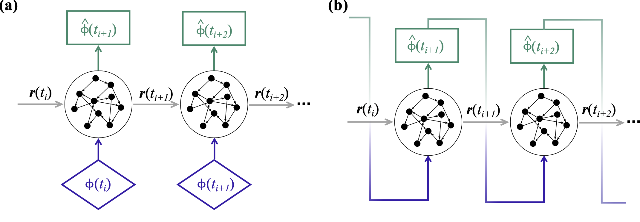
ESN open-loop and closed-loop configurations

Open-loop training and washout versus closed-loop forecasting.